TDM 40200 Project 13 - Introduction to Geospatial Data Analysis
Project and Learning Objectives
Make sure to read about, and use the template found on the template page, and the important information about project submissions on the submission page.
Dataset
-
/anvil/projects/tdm/data/fars/2021/accident.csv
-
/anvil/projects/tdm/data/tiger/state/tl_2021_us_state.zip
-
/anvil/projects/tdm/data/tiger/state/tl_2021_18_place.zip
The dataset used in this project is Fatality Analysis Reporting System (FARS), a US nationwide database tracking all fatal motor vehicle crashes, provided by National Highway Traffic Safety Administration (NHTSA). It can be useful in identifying and evaluating traffic safety problems and trends.
We also have more information under our FARS data page.
We also use the 2021 TIGER/LINE shapefiles from the US Census Bureau’s database that provides geospatial data on state and national boundaries, roads, and water features. Data obtained from catalog data page.
Additionally, the Indiana city data (used in Question 6) is from census gov page.
|
If AI is used in any cases, such as for debugging, research, etc., we now require that you submit a link to the entire chat history. For example, if you used ChatGPT, there is an “Share” option in the conversation sidebar. Click on “Create Link” and please add the shareable link as a part of your citation. The project template in the Examples Book now has a “Link to AI Chat History” section; please have this included in all your projects. If you did not use any AI tools, you may write “None”. We allow using AI for learning purposes; however, all submitted materials (code, comments, and explanations) must all be your own work and in your own words. No content or ideas should be directly applied or copy pasted to your projects. Please refer to GenAI page in the example book. Failing to follow these guidelines is considered as academic dishonesty. |
Questions
Geospatial data is numeric data that describes objects and events on specific locations on Earth. It consists of attributes such as characteristics of objects and time of occurrence, and coordinate information which are latitude and longitude.
We have been working with large datasets all the time; relevant to this, as data continues to grow larger, having an additional spatial dimension and information allow us to gain insights usually unobtainable from just numbers, for example variable changes or patterns across regions and boundaries, localized relationships or dependencies, and mapping and tracking.
For more reading, IBM website, titled "What is geospatial data?", has a good summary on what Geospatial data and analytics are with some applications.
Question 1 - (2 points)
EDA and Motivation
Let’s get familiar with the dataset and know the basic structure before getting started. First, please load in the 2021 data using:
df = pd.read_csv('/anvil/projects/tdm/data/fars/2021/accident.csv', encoding='latin1')Please print the head and shape of the dataset. Note the number of rows is the number of crashes.
# Head of the dataset
'''YOUR CODE HERE'''

# Shape of the dataset
'''YOUR CODE HERE'''
We now check for missing data to see if there are any unusual characteristics we should be aware of, or if any cleaning is needed.
# Check missing values for all columns
'''YOUR CODE HERE'''
You should see that it returns 0 for all the columns. At a first glance, it might look normal and all good to use, but try running:
print(df['LATITUDE'].value_counts().sort_index())
print(df['LONGITUD'].value_counts().sort_index())
Below will be the output values:
Latitude
|
Longitude
|
When you inspect the value counts for the coordinates, the sentinel values become immediately apparent at the end of the sorted index. Specifically, take a look at the last three values for both longitude and latitude. Does that make sense for a coordinate? Longitude can range from -180 to 180, and latitude can range from -90 to 90. The reason we see this is because NHTSA uses "sentinel values" instead of leaving null values. Variations of 7s represent "Not Reported", 8s represent "Not Applicable", and 9s represent "Unknown"; the last three values (77.777700 / 777700 and onwards) are the recoded numbers. "FARS/CRSS Coding and Validation Manual 2021" (and related documents) have detailed information on this.
Please print the number of the invalid latitude and longitude values in the dataset, and the number of normal, valid coordinates.
# Determine invalid latitude values
no_lat = (df['LATITUDE'] == 77.7777) | (df['LATITUDE'] == 88.8888) | (df['LATITUDE'] == 99.9999)

# Determine invalid longitude values
no_long = '''YOUR CODE HERE'''

print(f"\nNumber of missing/unknown latitude: {'''YOUR CODE HERE'''}")
print(f"Number of missing/unknown longitude: {'''YOUR CODE HERE'''}")
print(f"Normal coordinates: {'''YOUR CODE HERE'''}")-
In
no_lat, we check every row to see if latitude has the same value as the specified codes. We can do similar forno_long. The variables will containTruefor invalid data, andFalsefor valid data. -
Obtaining the number of normal coordinates can be done by calling
.sum(). Before that, we can use logical NOT to flip the 'True/False' values as not only do we want the valid counts, but also 'True' is what is counted by.sum().
You should get:
Number of missing/unknown latitude: 135
Number of missing/unknown longitude: 135
Normal coordinates: 39373
The total number of rows found in the beginning was 39508, and we can find from the current result that the invalid data accounts for approximately 0.3% of the entire data. It is fine to filter these out; additionally, not removing them could cause problems later with geographical visualization and analysis.
# Remove invalid data
df_clean = df[~no_lat & ~no_long].copy()
Please write code for below:
# Shape of the cleaned dataset
print(df_clean.shape)
# Range of values latitdue in this dataset take on
print(f"Latitude Range: {'''YOUR CODE HERE'''} to {'''YOUR CODE HERE'''}")
# Range of values longitude in this dataset take on
print(f"Longitude Range: {'''YOUR CODE HERE'''} to {'''YOUR CODE HERE'''}")-
We can use
.min()and.max()to obtain the lowest and highest values in a specific column.
Below is the expected output.
(39373, 80)
Latitude Range: 19.060325 to 66.89788333
Longitude Range: -162.59440556 to -67.2313
The shape matches our previous calculation since we dropped the 135 rows containing unusable location data. As well, the new latitude and longitude ranges correspond geographically with the actual US latitude and longitude (Approximately: Latitude southernmost at 18.91°N, northernmost at 71.44°N & Longitude 66.95°W to 172.46°E); sentinel values also cannot be contained in these ranges.
Lastly for this question, find the number of crashes per state:
print(df.groupby('STATENAME')['FATALS'].sum().sort_values(ascending=False))This results in list of fatality counts for all states, which one initially may think directly corresponds to the problem; however, this only gives us the pure count and no information on where. As well, crashes do not happen in an evenly spread manner within states, and we cannot obtain deeper insights with tables alone.
print(df[['STATENAME', 'LATITUDE', 'LONGITUD', 'FATALS']])-
Above selected the four columns ([[]] allows us to pick multiple specified columns simultaneously), and each row in the output represents a single event of a crash. The coordinates of where the crash happened is included here.
We need to utilize geographical information; coordinates in the data will help us bridge the regular dataset and table we started off with and spatial analysis.
-
1a. Code and corresponding documentation, and outputs for all required sections in the question.
-
1b. New cleaned dataset, output of its shape and required latitude and longitude values.
Question 2 - (2 points)
Introduction to Geospatial Data and GeoPandas
In our first question, we identified and cleaned coordinate data so now we have valid data to work with. If, for instance, we wanted to know where clusters occur for crashes, we would need geospatial tools. Clustering here refers to a technique that groups data points using similar geographical features and proximity.
Working with geospatial data in Python can be done by using the GeoPandas library. We can think of GeoPandas as a combination of the Pandas library and geometry. It has the abilites to perform spatial operations, geometric manipulations, and create maps.
Geometry Types
There are three main geometry types for Geospatial data
-
Points: Single (x,y) pair identifying a specific location.
-
Example: A crash that happened at a latitude/longitude.
-
-
Lines: Ordered set of connected coordinate pairs. Lines have length unlike points, but do not have an enclosed area like polygons do.
-
Example: A road.
-
-
Polygons: Series of points forming a closed loop.
-
Example: A state.
-
These are also the three basic geometric object classes in GeoPandas.
GeoDataFrame is an extension of the Pandas dataframe to accommodate geospatial vector data. It works the same way except there is an additional 'geometry' column storing shapes that represent Earth’s physical locations.
We already have GeoPandas on Anvil. Just import with:
import geopandas as gpdnew_df = gpd.GeoDataFrame(df_clean, geometry=gpd.points_from_xy(df_clean['LONGITUD'], df_clean['LATITUDE']), crs='EPSG:4326')-
gpd.GeoDataFrame(): returns the dataframe containing geometry. We passed in EPSG:4326 as 'crs' (Coordinate Reference System). EPSG:4326 is the "World Geodetic System 1984", which is the standard and the most widely used coordinate reference system. -
geometry=gpd.points_from_xy(df_clean['LONGITUD'], df_clean['LATITUDE']):.points_from_xy()takes in the longitude and latitude columns and converts into Point objects. It creates a GeometryArray directly.
|
When we say it gets converted into Point objects, the full detail is Shapely is a Python library meant to perform spatial operations on Cartesian plane (2D surface). It does not work with coordinate reference systems so for those aspects, it gets combined with GeoPandas. |
Print the type of the converted dataframe, which will confirm it.
# Type of new_df
'''YOUR CODE HERE'''
<class 'geopandas.geodataframe.GeoDataFrame'>
Then, print the full head, and head of the dataframe including only these columns: 'STATENAME', 'FATALS', 'LATITUDE', 'LONGITUD', 'geometry'.
For the second head print, you should see:
[5 rows x 81 columns]
  STATENAME  FATALS   LATITUDE   LONGITUD                    geometry
0   Alabama       2  33.601642 -86.312383  POINT (-86.31238 33.60164)
1   Alabama       2  33.541361 -86.643744  POINT (-86.64374 33.54136)
2   Alabama       1  33.419797 -86.752572   POINT (-86.75257 33.4198)
3   Alabama       1  33.360894 -86.777139  POINT (-86.77714 33.36089)
4   Alabama       1  33.815208 -86.825342  POINT (-86.82534 33.81521)
Note that the geometry column consists of values that looks like 'POINT (-86.31238 33.60164)'. These are shapely Point objects; geometry type is POINT which represents a single geographic location, with structure (longitude latitude).
Now that we have the points, we want to know and see the geographic context, which requires a map for plotting. Please load:
states_gdf = gpd.read_file('/anvil/projects/tdm/data/tiger/state/tl_2021_us_state.zip')As mentioned in the beginning of the project under the "dataset" section, this loads the US states boundary polygons from the Census Bureau’s TIGER dataset.
We can see the contents of the zipfile using Python’s zipfile module.
import zipfile

zf = zipfile.ZipFile('/anvil/projects/tdm/data/tiger/state/tl_2021_us_state.zip', 'r')
print(zf.namelist())
zf.close()-
namelist()in zipfile module returns a list of all file names inside zip.rtells zipfile to open the existing file for reading.
Below is the output, which are the list of files inside the zip file.
['tl_2021_us_state.cpg', 'tl_2021_us_state.dbf', 'tl_2021_us_state.prj', 'tl_2021_us_state.shp', 'tl_2021_us_state.shp.ea.iso.xml', 'tl_2021_us_state.shp.iso.xml', 'tl_2021_us_state.shx']
GeoPandas detects that we have a ZIP and scans content for datasets and finds the shapefile components. Here it consists of multiple files like .shp, .shx, .dbf together storing geometry and attribute data; they are read together as one data, and are loaded into a GeoDataFrame.
Please print the head and shape of this dataframe.
# Shape
print(f"states_gdf shape: {'''YOUR CODE HERE'''}")
# Head
'''YOUR CODE HERE'''
Also please check the CRS of both states_gdf and new_df using .crs.
# Print CRS of states_gdf
'''YOUR CODE HERE'''
# Print CRS of new_df
'''YOUR CODE HERE'''
It outputs:
EPSG:4269
EPSG:4326
EPSG:4326 (WGS 84) and EPSG:4269 (NAD83) are both coordinate systems that uses latitude and longitude, but WGS84 is the standard global system that is based on the center of mass of the Earth, while NAD83 is catered towards North America. The coordinates are very close to each other, but there are small numerical differences.
GeoPandas generally cannot correctly plot two dataframes with different CRS, as alignment between layers will not be correct. To prevent problems, we use .to_crs() which lets us change the coordinate reference system for all points in all objects.
states_gdf = states_gdf.to_crs('EPSG:4326')Print the head of states_gdf. Notice in the 'geometry' column, we now have 'POLYGON' and 'MULTIPOLYGON' objects instead of Points. Multipolygon is another geometry type in GeoPandas describing a single geographical feature made of separate polygons; here in another words, states with islands or some separated area but still a part of that state (for example, Florida or Hawaii).
Also, re-print `state_gdf’s crs to confirm.
print(f"New states_gdf crs: '''YOUR CODE HERE''' ")We will create our first plot soon, but before that we should further inspect the column and understand geometry object. Let’s select one state (we picked Indiana here because Purdue is in Indiana! But feel free to pick a state of your choice).
Please complete the code, and see below the code block for more guidance.
indiana = states_gdf[states_gdf['NAME'] == 'Indiana'].iloc[0]
# Print state name
print(f"State: {indiana['NAME']}")
# Print geometry type
print(f"Geometry type: {indiana.geometry.geom_type}")
# Print bounding box
print(f"Bounding box: {indiana.geometry.bounds}")-
The first line filters for 'Indiana' and we use
.iloc[0]to get the first matching row as a spatial series (and not one row dataframe). -
State name can be printed by accessing the column as usual.
-
Finding the geometry type: As mentioned, spatial data is stored in GeoPandas' special column 'geometry'. Look into
.geometryand you can use that in the code. Since Indiana here is a single row, it will directly access that object..geom_typereturns the type of geometry. -
Finding bounding box: You can use
.bounds()here. It returns a tuple (minx, miny, maxx, maxy), which are westernmost longitude, southernmost latitude, easternmost longitude, and northernmost latitude, respectively. A polygon’s boundary is a sequence of coordinate paris.
State: Indiana
Geometry type: Polygon
Bounding box: (-88.097892, 37.771672, -84.784535, 41.761368)
Above is the result for Indiana. We can see that it is represented as a single polygon, so it has continuous boundary and no separate area belonging to the state. In GeoPandas, we can also obtain the list of all coordinates at the boundary using .GeoSeries.exterior; polygons can have an exterior (outer boundary) or interiors (boundaries of any holes inside), and this selects the outer part. We can then obtain raw coordinate sequences using .coords (get list of all dots that make up the outer ring). Use this information to find the number of coordinates at the border.
print(f"Number of coordinates of Indiana border: {'''YOUR CODE HERE'''}")Number of coordinates of Indiana border: 16235
As we can see, Indiana border is defined by 16235 pairs. We note, first this is another way to see that the dataset itself is high resolution that captures many small details. Secondly, the high numbers make sense considering the parts of Indiana borders that are very bent and not linear; more bend there is, more (x,y) would be needed in the exterior.coords list.
Plotting
Now, we layer the two GeoDataFrames on the same matplotlib axes. We will put polygons in the background and points on top.
fig, ax = plt.subplots(figsize=(10, 6))

states_gdf.plot(ax=ax, color='silver')
new_df.plot(ax=ax, color='red', markersize=0.2)

ax.set_title('All Fatal Traffic Crashes — 2021')
plt.show()-
states_gdf.plot(ax=ax, color='silver'): This draws the state boundaries onto the created axes. -
new_df.plot(ax=ax, color='red', markersize=0.2): This is for the point layer. We put this line after the state plot, allowing us to draw dots on top of the state shapes. Additionally, setting the markersize lower can help us see individual points and density a little more clearly, since we have a huge number of total crashes and large dots would overlap.
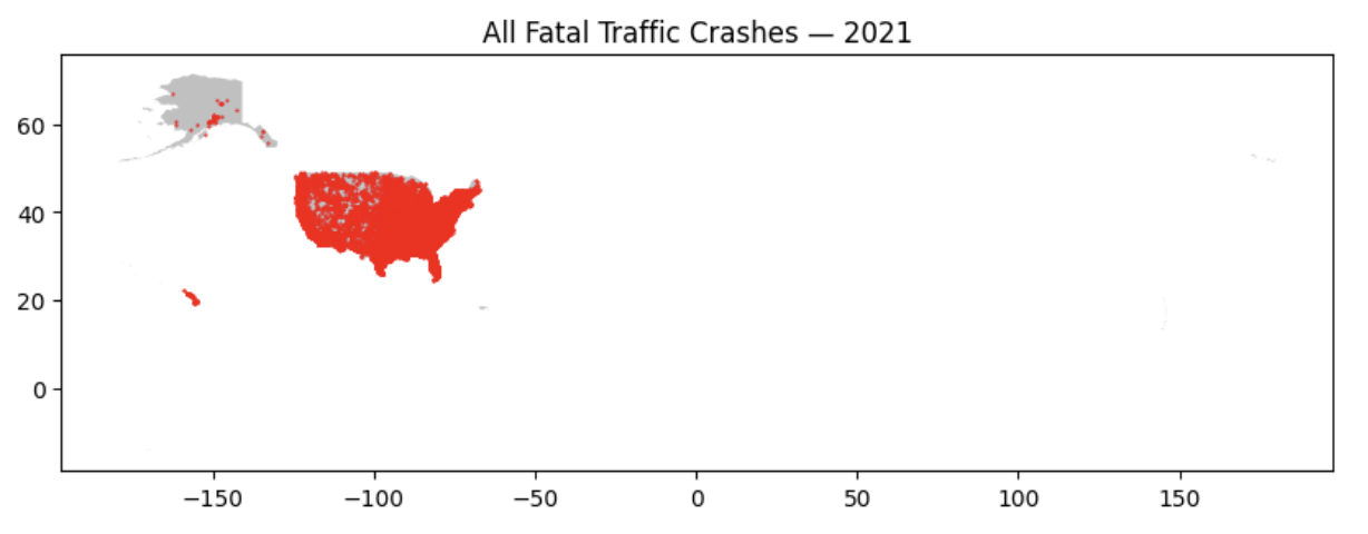
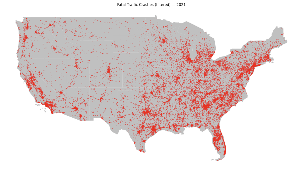
Notice the map covers a very large area because we are including all locations, territories, and states of the USA. This makes the map very zoomed out. Below we filter out noncontiguous states and territories for visual scaling.
fig, ax = plt.subplots(figsize=(14, 8))

# Only showing contiguous states (excluding noncontiguous and territories)
to_exclude = ['Alaska', 'Hawaii', 'American Samoa', 'Guam','Commonwealth of the Northern Mariana Islands','Puerto Rico', 'United States Virgin Islands']

contiguous_states = states_gdf[~states_gdf['NAME'].isin(to_exclude)]

accidents = new_df[~new_df['STATENAME'].isin(['Alaska', 'Hawaii', 'Puerto Rico'])]

# State (background)
'''YOUR CODE HERE'''

# Crash points
'''YOUR CODE HERE'''

# Title and output of the map
'''YOUR CODE HERE'''-
contiguous_states: We select the NAME column from the dataframe and use.isin(to_exclude)to check if each value is in the 'to_exclude' list; it produces boolean series where 'True' values will be excluded. Since we will use indexing to only keep the rows with true condition, logical NOT is used to change the true/false values. Thus, this results is all states except the ones listed in 'to_exclude'. 'accidents' works in a similar way.
|
FARS dataset includes: 50 U.S. states, the District of Columbia, and Puerto Rico. TIGER dataset includes: All of the United States and associated territories We exclude what is actually present in the data. |
You will get the following map:
-
2a. Code and corresponding documentation, and outputs for all required sections in the question.
-
2b. Written explanation on your observation and findings from the map outputs. What information do we obtain?
Question 3 - (2 points)
Spatial Join and Map
We found where crashes occurred in the map in question 2. In order to find out where we get the most crashes, we connect the points to the polygon it belongs inside. We can do this with GeoPandas' .sjoin().
Spatial join combines two datasets by matching rows by spatial relationship (similar to merge in pandas, but here we are not matching by common attribute value), for example which polygon contains a point, if there is an intersection, and proximity.
crash_joined = gpd.sjoin(accidents, contiguous_states, how="inner", predicate='within')-
accidentsis the left/primary dataset which are the points we want to keep, andcontiguous_statesis the right/reference dataset where we get the information from and attach it to the points. -
We then define some rules.
how="inner"keeps the rows that finds a match only.predicate='within'means the point must be inside the polygon.
Please complete code below.
new_col = []
for c in crash_joined.columns:
  # Check if the column name is not already in `accidents.columns`
  '''YOUR CODE HERE'''
    # append to new_col
    '''YOUR CODE HERE'''

print(f"Columns added: {new_col}")
Columns added: ['index_right', 'REGION', 'DIVISION', 'STATEFP', 'STATENS', 'GEOID', 'STUSPS', 'NAME', 'LSAD', 'MTFCC', 'FUNCSTAT', 'ALAND', 'AWATER', 'INTPTLAT', 'INTPTLON']
All the columns above came from 'contiguous_states'
Also, especially note
|
TIGER Technical Documentation 2021 is a good reference to find more information on how geographic data is structured, coded, and used. This includes some definitions, attribute tables, and relationships that may be helpful. |
Print the head of the joined data. We can immediately see from first few rows that they are Alabama crashes; take a look at some columns, including ALAND (land area), AWATER (water area), INTPTLAT/INTPTLON (Current latitude of the internal point), and we can also observe they all have Alabama specific attributes (for example, ALAND = 131175477769 in square meters - consistent with Alabama’s known square miles size of approx. 50,750).
crashes_per_state = (crash_joined.groupby('NAME').agg(crash_cnt=('ST_CASE', 'count'),
                                                      total_fatals=('FATALS', 'sum'),
land_area=('ALAND', 'first')).reset_index())-
We first grouped the dataset by 'NAME' column so that rows are grouped together if they belong in the same state.
-
.agg()is used to get the statistic for each group. Here we create three new columns:-
crash_cntcounts the number of rows/crashes per state. 'ST_CASE' is a unique case identifier. -
total_fatalsgets the total fatalities in each state. -
land_areagets the land area of each state. We chose the first value, since all rows in the same state will have the same land area, and we just need to get one.
-
# Print top 10 states by crash counts
'''YOUR CODE HERE'''
The output will be:
              NAME  crash_cnt  total_fatals     land_area
41           Texas       4066          4495  676681550479
3       California       3970          4271  403671756816
8          Florida       3444          3731  138961722096
9          Georgia       1670          1797  149486624386
31  North Carolina       1525          1653  125933327733
33            Ohio       1242          1354  105823653399
40       Tennessee       1229          1327  106791957894
11        Illinois       1205          1329  143778561906
36    Pennsylvania       1152          1229  115881784866
38  South Carolina       1112          1198   77866200776
Texas has the highest number of fatal crashes, followed by California, Florida, and so on. To visualize this, we can merge the statistic with geographic boundaries and plot a choropleth. Different geographic regions will be shaded based on the value of a variable. In this case, the states will be coloured depending on the number of fatal crashes; spatial patterns or clusters will be easily identified.
# Merge statistics back with map shapes
states_with_stat = '''YOUR CODE HERE'''

fig, ax = plt.subplots(figsize=(10, 6))

# Plot choropleth
states_with_stat.plot(column='crash_cnt', ax=ax, legend=True,edgecolor='white', linewidth=0.5)

# Map output
'''YOUR CODE HERE'''-
To do:
-
Use
.merge()to combine 'contiguous_states' and 'crashes_per_state' (get state shapes & crash statistic from each). You should keep all states in the map dataset and add in the crash data where we have it. -
Output the map and add in labelling/title. Note: Mapping and plotting tools guide has good introduction to more plotting/mapping tools.
-
It will look like:
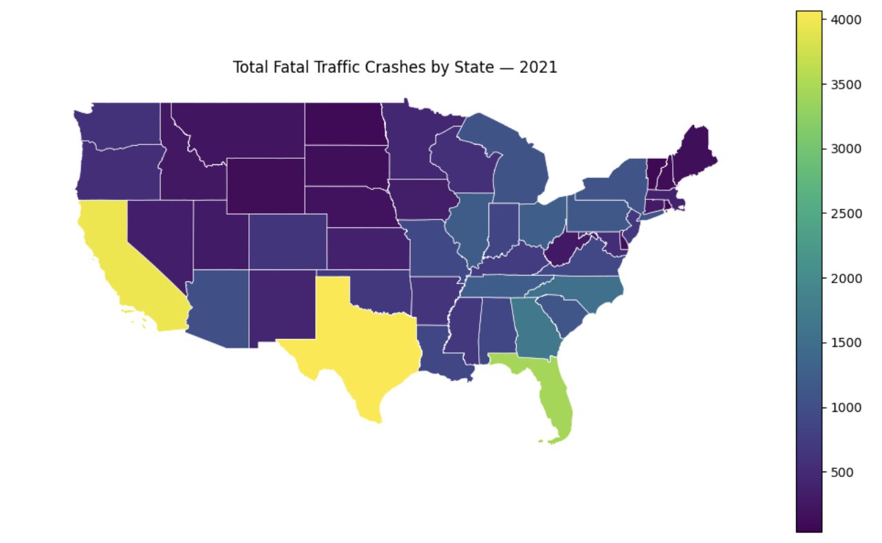
It shows us geographic distribution of fatal crashes across US states. The lighter colours denote states with higher raw crash counts, and the pattern for this is quite clear. The states with these colours are also the states with highest population in the country. Conversely, states in areas such as upper midwest show the opposite result.
-
3a. Code and corresponding documentation, and outputs for all required sections in the question.
-
3b. Write a few sentences on your own understanding of how we obtained
crash_joined, your interpretation of resulting data and where it could be useful. As well, what are your observations are from printing the head (you are free to explore and take a look at other attributes and outputs as well)? -
3c. Write about your interpretation of the choropleth. Also, are there any patterns? Do you think there are limitations to what we have right now and information it conveys?
Question 4 - (2 points)
While the map using raw count is useful for total volume, there can be bias incorporated; states such as Texas and California inherently will have more crashes as they are a lot more populated with larger land area and road and infrastructure counts. So to make comparison, we will normalize and create our visualization using density.
We will use 'ALAND' (land area) column we obtained from joining. It will first be converted to square km just for managing the numbers and readability.
# Convert sq m -> sq km
crashes_per_state['land_area_sqkm'] = crashes_per_state['land_area'] / 1000000
Now we calculate the density measuring how concentrated the fatal crashes are in each state.
# Crashes per 1000 sq km
crashes_per_state['crash_density'] = (crashes_per_state['crash_cnt'] / crashes_per_state['land_area_sqkm']) * 1000-
crash_cnthas the total number of fatal crashes in the state andland_area_sqkmhas the size of the state in square kilometers. Divide and we get crashes per square km. The last multiplication by 1000 scales it to per 1000 sq km, which is better for reading and comparing.
Please write the code to sort by either crash_cnt or crash_density column and make the highest values be shown first. Print the first 10 rows after.
print("Top 10 States for Crash Count")
'''YOUR CODE HERE'''

print("\n Top 10 States for Crash Count - Density (per 1000 sq km)")
'''YOUR CODE HERE'''
The second print output shows:
 Top 10 States for Crash Count - Density (per 1000 sq km)
                    NAME  crash_cnt  total_fatals     land_area  \
7   District of Columbia         36            37     158316124
28            New Jersey        667           697   19048916230
6               Delaware        131           135    5046731559
8                Florida       3444          3731  138961722096
5            Connecticut        283           298   12541690473
37          Rhode Island         60            62    2677763359
18              Maryland        526           565   25151992308
19         Massachusetts        397           417   20204390225
38        South Carolina       1112          1198   77866200776
31        North Carolina       1525          1653  125933327733

    land_area_sqkm  crash_density
7       158.316124     227.393137
28    19048.916230      35.015115
6      5046.731559      25.957394
8    138961.722096      24.783803
5     12541.690473      22.564741
37     2677.763359      22.406760
18    25151.992308      20.912856
19    20204.390225      19.649195
38    77866.200776      14.280907
31   125933.327733      12.109582
We had Texas as the highest raw crash count previously, but here it disappeared from the top 10 list. Texas is geographically very big which makes crashes spread out over a large area. On the other hand, smaller states such as New Jersey and onwards were never seen and now they took over the top 10 list; they are geographically small but have a much denser infrastructure and high traffic volumes, so while the total crashes is lower, they can have higher concentration of incidents per square km. Lastly, District of Columbia appears as a bit of an outlier in density results due to its very small land area compared to other states; since the calculation used division of number of crashes by land area, even small number of crashes is amplified. This could lead to some sensitivity.
Try creating a mapped visualization for this, similar to what we did in question 3.
# Merge with map shapes (crashes_per_state)
density_map = '''YOUR CODE HERE'''

fig, ax = plt.subplots(figsize=(10,6))

density_map.plot(column='crash_density', ax=ax, legend=True, edgecolor='white', linewidth=0.5)

# Map output with label/title
'''YOUR CODE HERE'''
You will see that the map is generally same coloured with not much variation at all. This is not necessarily a data problem, but a scaling problem in visualization. Remember there was one data point significantly higher than the rest (DC); since a linear scale was used, all other values get compressed into the same bin for colouring. We can use norm=plt.matplotlib.colors.LogNorm(), which transforms into a log scale, to fix the visualization.
density_map.plot(column='crash_density', ax=ax, legend=True, edgecolor='white', linewidth=0.5, norm=plt.matplotlib.colors.LogNorm())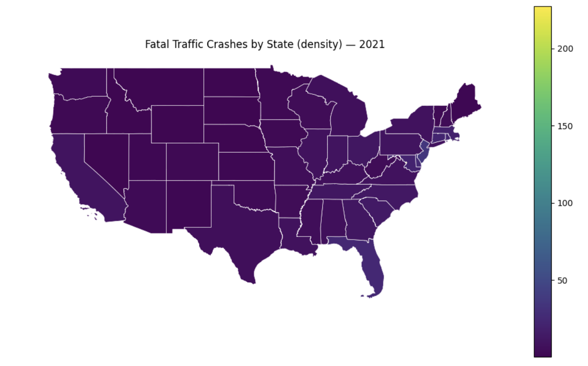
Figure 4. Original
|
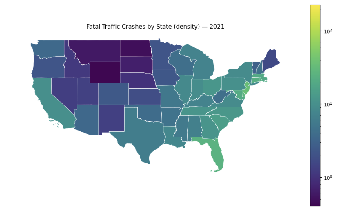
Figure 5. After scaling
|
Now there are distinct shades across states that were not visible previously.
-
4a. Code and corresponding documentation, and outputs for all required sections in the question.
-
4b. Take a look at the result for District of Columbia and write a few sentences on your interpretation. In this case and in general, are there any outliers? What is causing DC to have unusual numbers?
-
4c. Map outputs of both before and after scaling. Can this change spatial interpretation of fatal crash across states?
Question 5 (2 points)
In previous questions, we looked at crash patterns and information at the state level, but there exists localized variations within a state. For instance, crashes in urban areas could differ from those occurring on rural places. To address this, we will examine pattern in a single state.
Local Focus
Let’s filter our data to Indiana only and look at the crash distribution. We will colour each crash point by whether it happened on a rural or urban road using the RUR_URB column (this indicates whether crash happened in a rural or an urban setting).
Below code will first tell us how many crashes happened in Indiana, and how they are split between rural and urban locations.
# Crashes in indiana only
indiana_crashes = accidents[accidents['STATENAME'] == 'Indiana'].copy()
# Indiana only state boundary
indiana_boundary = contiguous_states[contiguous_states['NAME'] == 'Indiana']

# Number of crashes in indiana_crashes
print(f"Number of fatal crashes in Indiana (2021): '''YOUR CODE HERE'''")

# Description of what we are printing below
'''YOUR CODE HERE'''

# Rural and Urban crashes counts
'''YOUR CODE HERE'''-
indiana_crashesis a filtered dataset with just Indiana rows. -
For rural and urban crash counts, look at the column
RUR_URB, and we can usevalue_counts().
Now we visualize both on the same map.
fig, ax = plt.subplots(figsize=(8, 7))

# Put indiana state boundary as the background
indiana_boundary.plot(ax=ax, color='whitesmoke')

# Crashes by rural & urban + different colours
rural = indiana_crashes[indiana_crashes['RUR_URB'] == 1]
urban = indiana_crashes[indiana_crashes['RUR_URB'] == 2]

rural.plot(ax=ax, color='slategrey', markersize=3, label='Rural')
urban.plot(ax=ax, color='lightsteelblue', markersize=3, label='Urban')
We can also add a legend manually; to do this, we use:
import matplotlib.patches as mpatchesPatches are geometric shapes we can draw on plot in matplotlib. This allows us to create patches and put in legend. In below code, we use in 'legend_elements' to define each parts and corresponding colours. We could create legends automatically, but this is another way to do it while having more control over placement and design, especially if we want to be specific in a more complex plot.
# Legend
legend_elements = [mpatches.Patch(color='slategrey', label=f'Rural ({len(rural)} crashes)'),
                   mpatches.Patch(color='lightsteelblue', label=f'Urban ({len(urban)} crashes)')]

ax.legend(handles=legend_elements)

# Map output with label/title
'''YOUR CODE HERE'''
The code chunk above creates a list of legend elements. By using mpatches.patch(), Matplotlib knows to create coloured box in the legend. You can see the parameters where we can choose the legend colour box and label; we can also do custom formatting (it allows fstrings, value modifications, and getting certain stats like len()).
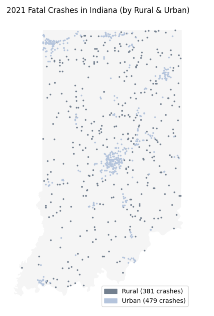
Some things we can notice include the way they cluster. Urban crashes seem to be more merged around major population and transportation areas, while rural crashes are more spread out across the state; also, a lot of them are most likely occurring near highways or longer distance roads with attributes such as higher speed limits.
Now let’s compare the fatality rates, and find out which of the two are more fatal on average. Please print the average fatality per crash for both areas.
rural_fatal = '''YOUR CODE HERE'''
urban_fatal = '''YOUR CODE HERE'''

print(f"Average fatalities (rural): {'''YOUR CODE HERE'''}")
print(f"Average fatalities (urban): {'''YOUR CODE HERE'''}")-
For
rural_fatal, use the dataset filtered to rural crashes only, and select the column that shows the death/fatal counts per crash. Then, compute average value. Use similar idea forurban_fatal, but only using urban rows and its statistic.
You will see below statistic:
Average fatalities (rural): 1.1128608923884515
Average fatalities (urban): 1.0542797494780793
Rural crashes have higher average fatalities per incident compared to that of urban crashes. Taking real world scenario into account, we could infer they could be caused by factors such as higher speed limits as mentioned previously, less access to safety features and emergency responders, and varying road conditions.
Please print all unique values in the 'REGION' column of states_gdf.
print('''YOUR CODE HERE''')US Census Bureau has geographic region definition that uses single integer value to represent four US regions: Northeast, Midwest, South, and West.
Original Region Codes:
['3' '2' '1' '4' '9']
-
'9' is not part of the four standard regions, and we can think of them as unidentified by state or some other entry.
We will combine the crash stats with state geometry/boundaries. Below merge matches rows using 'NAME' (state name) and keeps all states in contiguous_states and add in the crash data.
states_region = contiguous_states.merge(crashes_per_state, on='NAME', how='left')Since coded values were used originally for each regions, we create readable region names. Below is a dictionary mapping numeric region codes to labels, where 1 = Northeast, 2 = Midwest, 3 = South, and 4 = West.
region_names = {'1': 'Northeast', '2': 'Midwest', '3': 'South', '4': 'West'}
states_region['REGION_NAME'] = states_region['REGION'].map(region_names)
# Head of states_region
'''YOUR CODE HERE'''You will notice the the mapping operation is reflected. Take a look at REGION and REGION_NAME columns. For example, West Virginia has region 3 and the assigned name is South. You might also be able to infer some other information regarding how high or low crash counts and density are between regions relatively.
Now, we will use GeoPanda’s .dissolve() . A way to think of it is like performing groupby with shapes. As the name suggests, it merges geometries within a group into one feature and aggregates all rows in a group.
regions_gdf = states_region.dissolve(by='REGION_NAME',
                                       aggfunc={'crash_cnt': 'sum',
                                                'total_fatals': 'sum',
'land_area': 'sum'}).reset_index()-
states_region.dissolve(): As mentioned, this groups geometries and data based on category.-
We used
by='REGION_NAME', meaning all states with same region name are grouped and combined into one geometry. -
By using a`ggfunc={}`, we add all states for each of the three columns -
crash_cnt,total_fatals, andland_area. We obtain the regional total.
-
Print regions_gdf, and you will get:
  REGION_NAME                                           geometry  crash_cnt  \
0     Midwest  POLYGON ((-98.34819 36.99815, -98.34874 36.998...       7454
1   Northeast  MULTIPOLYGON (((-74.48282 39.28414, -74.48695 ...       3949
2       South  MULTIPOLYGON (((-80.18532 25.33851, -80.18697 ...      19394
3        West  MULTIPOLYGON (((-118.65436 33.07495, -118.6413...       8423

   total_fatals      land_area
0          8126  1943991852468
1          4185   419354636236
2         21156  2249835530078
3          9169  3041775201247
Now, we are at the last step of normalizing and creating visualization; we will be able to compare regions visually. Please complete the code below. The process will be quite similar to what we did previously.
# Convert land area from sq m to sq km
regions_gdf['land_area_sqkm'] = '''YOUR CODE HERE'''

# Calculate density with (total crashes/total area) * 1000
regions_gdf['crash_density'] = '''YOUR CODE HERE'''

# Print result highest to lowest
'''YOUR CODE HERE'''
Then print the regional choropleth map, which will result in:
fig, ax = plt.subplots(figsize=(10,6))

regions_gdf.plot(column='crash_density', ax=ax, legend=True, edgecolor='white', linewidth=0.5)

ax.set_title('Fatal Crash Density by Region — 2021')
ax.set_axis_off()
plt.tight_layout()
plt.show()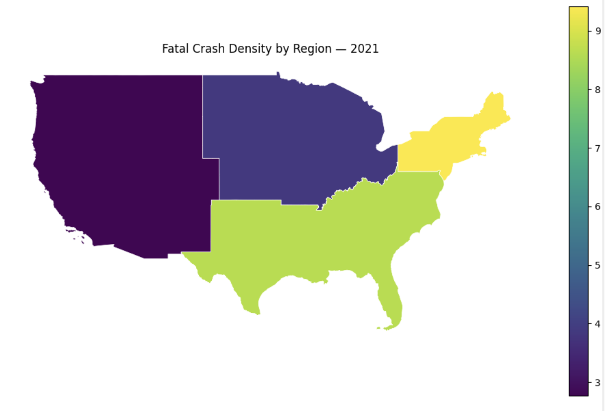
-
5a. Code and corresponding documentation, and outputs for all required sections in the question.
-
5b. Write a few sentences on your findings from the urban & rural map. What differences do you notice and what do you think the reasons are? Do you think this is related to fatality rates, and why?
-
5c. Print
regions_gdfand what insights can you get from the dataset initially?
Question 6 (2 points)
So far, we have analyzed the number of crashes that occurred in various areas; it may be a natural question to ask how far crashes are from a given location or object.
CRS for measurement
We have been using EPSG:4326 for coordinates in degrees, meaning we cannot compute accurate distances. For measurements, we will reproject the CRS to use meters. Here, we picked EPSG: 32616 (WGS 84 / UTM zone 16N), which is a valid choice for US midwestern states (contains Indiana and closer neighbouring states, and more specifically, approx. longitude 90°W and 84°W).
indiana_crashes_new = '''YOUR CODE HERE'''
indiana_boundary_new = '''YOUR CODE HERE'''

# Print original and new CRS
print(f"Original CRS: '''YOUR CODE HERE'''")
print(f"Projected CRS: '''YOUR CODE HERE'''")

# Sample for comparison
print(f"\nBefore: {indiana_crashes.geometry.iloc[0]}")
print(f"After: {indiana_crashes_new.geometry.iloc[0]}")
You will see the following output:
Original CRS: EPSG:4326
Projected CRS: EPSG:32616

Before: POINT (-86.87769444 40.76559167)
After: POINT (510322.44120885874 4512743.238172149)
Clearly, the values changed from smaller real values representing decimal degrees, to larger values representing meters. These are distances in meters from the UTM zone; any calculations we do with these will be meter based results.
TIGER - PLACES
In the TIGER database, the cities and their boundaries are found under Places, whose shapefiles contains data on cities, towns, etc, as well as Census Designated Places.
# Indiana city data
places = gpd.read_file('/anvil/projects/tdm/data/tiger/state/tl_2021_18_place.zip')
The Federal Information Processing Standard (FIPS) code for Indiana is 18, hence you see the dataset specificed with the code '18'. The code uniquely identifies state and its county level data.
|
FIPS, established by the National Institute of Standards and Technology (NIST), is public standard and guidelines for US federal computer systems. There are many categories, including Cryptography, Data Standards and Codes, Computer Graphics, and Personal Identity Versification, and so on. |
Please print the shape, CRS, list of columns, and the head of the places dataset.
print(f"Shape: {'''YOUR CODE HERE'''}")
print(f"CRS: {'''YOUR CODE HERE'''}")
print(f"\nColumns: {'''YOUR CODE HERE'''}")

# Head
print('''YOUR CODE HERE''')
The CRS output will show 'EPSG:4269'. As we have already seen, this uses degrees and we cannot calculate the distance to a nearest point using this, so we will reproject to 'EPSG:32616' later on.
As well, the shape will be 'Shape: (696, 17)'; we have hundreds of places in the shapefile. Since this is too many for all to be used as reference points, we will filter for major cities.
cities = places[places['NAMELSAD'].str.contains('city', case=False)].copy()

print(f"Included Indiana Cities: {len(cities)}")

# Sort by land area to find major cities
cities = cities.sort_values('ALAND', ascending=False)

print("\nCities sorted by land area:")
print(cities.head(10))
Now, please write the code to pick top 10 cities largest by land area and save into selected_cities. Then, print only the 'NAME' and 'ALAND' of the selected cities.
# Pick top 10 for reference
selected_cities = '''YOUR CODE HERE'''

print("Selected Indiana Cities (major by area):")
print('''YOUR CODE HERE''')
Computing centroids for cities
Indianapolis, for example, is an irregular shape for city boundary. If we wanted to calculate distances, we would need a consistent, representative point. We can do so by using centroid, which is the geometric center of a polygon. This can be obtained automatically by GeoPandas. Before we do that, as previously mentioned, please convert the CRS to 'epsg=32616'.
# Convert selected_cities CRS to 'epsg=32616'
selected_cities = '''YOUR CODE HERE'''
Now, we compute centroids for the cities. Specifically, we can do so by using .geometry to access the geometry column, and .centroid to obtain the points representing the center of the region.
# Get centroid for each cities
selected_cities['centroid'] = selected_cities.geometry.centroid
Please print the name and centroid in selected_cities.
print("City centroids - projected meters:")
print('''YOUR CODE HERE''')
Output:
City centroids - projected meters:
                            NAME                        centroid
196  Indianapolis city (balance)  POINT (573153.496 4403364.483)
489                   Fort Wayne  POINT (655915.466 4550270.251)
394                         Gary   POINT (471076.43 4604389.176)
560                       Carmel  POINT (572932.547 4424224.527)
559                   Evansville  POINT (453099.996 4204627.189)
304                   South Bend  POINT (560801.511 4614135.625)
257                     Anderson  POINT (611740.388 4438470.521)
47                        Kokomo  POINT (573953.711 4479618.411)
405                      Fishers  POINT (588311.842 4423692.218)
333                  Terre Haute   POINT (467612.024 4368455.34)
Similarly as before, we no longer have latitude and longitude but values in meters. The first numbers is the distance from the central meridian of UTM zone, and the second number is the distance from the Equator.
Let’s create a visualization to see the centroids for each cities!
# Visualization of cities and their centroids:

fig, ax = plt.subplots(figsize=(8, 7))

indiana_boundary_new.plot(ax=ax, color='whitesmoke')

# Cities
selected_cities.plot(ax=ax, color='lightsteelblue')

# Centroids: use red on top
selected_cities['centroid_geom'] = selected_cities.centroid
centroids_gdf = selected_cities.set_geometry('centroid_geom')
centroids_gdf.plot(ax=ax, color='red', markersize=10)

# Labelling
# Iterate through each rows (each city)
for _, row in selected_cities.iterrows():
    # Geometric center of current shape
    centroid = row.geometry.centroid
    # Place at (x,y) the city name
    ax.text(centroid.x, centroid.y, row["NAME"], fontsize=7)

ax.set_title('Major Indiana Cities & Centroids')
ax.set_axis_off()
plt.tight_layout()
plt.show()
See below for more explanation of this section of the code:
-
We build the map in layers again. the base layer is the polygon shape of Indiana on
ax. Then, on the same axes we plot the city boundaries. This results in subregions layers on top of a larger region. -
selected_cities['centroid_geom'] = selected_cities.centroid-
This computes the centroid of each city, and stores the result in
centroid_geomcolumn.
-
-
centroids_gdf = selected_cities.set_geometry('centroid_geom')-
We normally have the geometry column storing shapes. Here we create a second geometry to have a column with points (
centroid_geom).set_geometrylets us change the currently used geometry column from 'geometry' to the specific, here 'centroid_geom'. So,centroid_gdf.plot()will plot points (compared to, for example,selected_cities.plot()will plot polygons).
-
-
To add labels to our map, we iterate through all rows (with
.iterrows()), where each row corresponds to a city; this works sinceselected_citiesis a GeoDataFrame. Then, the first line inside the for loop states to obtain the geometric center of the current shape.row.geometryaccesses the geometry object for the specific row, and.centroidreturns a point geometry after computing the center; so the input is the city boundary which is a polygon, and the output is a single point. This leads to why we are able to access the x and y values in the coordinate of 'centroid' in the second line.
We obtain the below map:
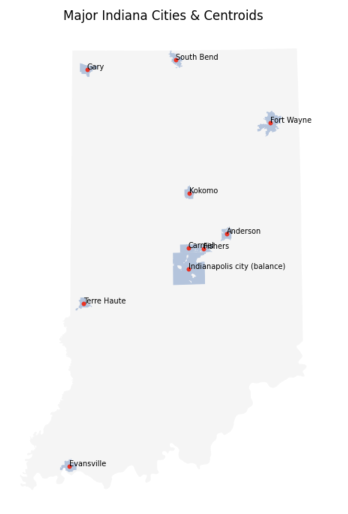
The blue polygons are TIGER provided city boundaries, and the red dots are computed centroids.
Distance - Crash & Nearest City
We will now explore distance calculation and sjoin_nearest() by using the centroids to see how far Indiana crashes occurred from nearest major city.
# Dataframe
city_centroids_gdf = selected_cities.set_geometry('centroid')[['NAME', 'centroid']].copy()

# Rename city column (NAME to nearest_city)
city_centroids_gdf = city_centroids_gdf.rename(columns={'NAME': 'nearest_city'})

crashes_nearest = gpd.sjoin_nearest(indiana_crashes_new, city_centroids_gdf, how='left', distance_col='dist_nearest_m')

crashes_nearest['dist_nearest_km'] = crashes_nearest['dist_nearest_m'] / 1000-
We had
selected_cities, with city polygons as geometry and point column as centroid. Here, by doingset_geometry('centroid'), we allow all operations to use these centroid points. Then, since we just need the locations for distance, we kept just the city name and point geometry with[['NAME', 'centroid']]. -
sjoin_nearestingpd.sjoin_nearest(indiana_crashes_new, city_centroids_gdf, how='left', distance_col='dist_nearest_m').-
sjoin_nearestfinds the closest city centroid for each crash point. Each geometry in the left dataset is compared to all geometries in the right dataset (so each crash compared to each centroid), then distances are computed with the smallest one picked. -
how='left'keeps all crash points. Output size is the number of crashes. -
Distance between the crashes and their nearest centroids are computed by GeoPandas. 'distance_col='dist_nearest_m'' stores the values in the new column
dist_nearest_m.
-
|
Naive approach to this computation would be using nested loop: for each crash, for each city, compute the distance and pick the smallest. This however is very inefficient, especially with large datasets. Using |
Print and inspect the head after this part.
Then, find which city appears most as the nearest city for crashes. In another word, how many times does each city appear in crashes_nearest?
# Which city appears most as nearest?
print("Cities appearing most:")
print('''YOUR CODE HERE''')
We now create a spatial visualization to see how these distances are distributed across the state.
indiana_crashes = indiana_crashes.copy()
indiana_crashes['dist_nearest_km'] = crashes_nearest['dist_nearest_km'].values
indiana_crashes['nearest_city'] = crashes_nearest['nearest_city'].values
crashes_nearest had meters coordinates and not degrees, so we copy computed distances back onto the original dataframe.
fig, ax = plt.subplots(figsize=(8, 7))

# Indiana boundary as background
indiana_boundary.plot(ax=ax, color='whitesmoke')

# Crash points coloured by distance
scatter = ax.scatter(indiana_crashes['LONGITUD'], indiana_crashes['LATITUDE'], c=indiana_crashes['dist_nearest_km'], s=2)
In question 5, we plotted a fixed colour (one each for rural and urban), but here we will use ax.scatter(.. c=) to map distance which takes on continuous values.
-
indiana_crashes['LONGITUD'], indiana_crashes['LATITUDE']: These provide the x, y coordinates for each point. -
c=indiana_crashes['dist_nearest_km']: Colour is assigned to each point determined by distance. Low and high values get mapped to each ends of the colourmap. -
s=2: Since there are hundreds of points and some overlapping, we set the point size to be smaller for visual purposes.
# City centroid
selected_cities_conv = selected_cities.to_crs(epsg=4326)

# Place marker and label for each city
for _, row in selected_cities_conv.iterrows():
    cx = row.geometry.centroid.x
    cy = row.geometry.centroid.y
    ax.scatter(cx, cy, color='red')
ax.annotate(row['NAME'], (cx, cy), fontsize=8)-
Here, we convert back to EPSG:4326, ensuring cities and crash points align by using degrees.
-
For loop:
-
'cx', 'cy' gets the x,y (longitude, latitude) values of the city’s center
-
For reference, we want to show the center with city label, and
ax.scatter(cx, cy, color='red')draws a red dot at the centroid for us. -
ax.annotate(row['NAME'], (cx, cy), fontsize=8)writes the city name by the dot; row['NAME'] and (cx,cy) provides the text and position respectively.
-
The map will look like:
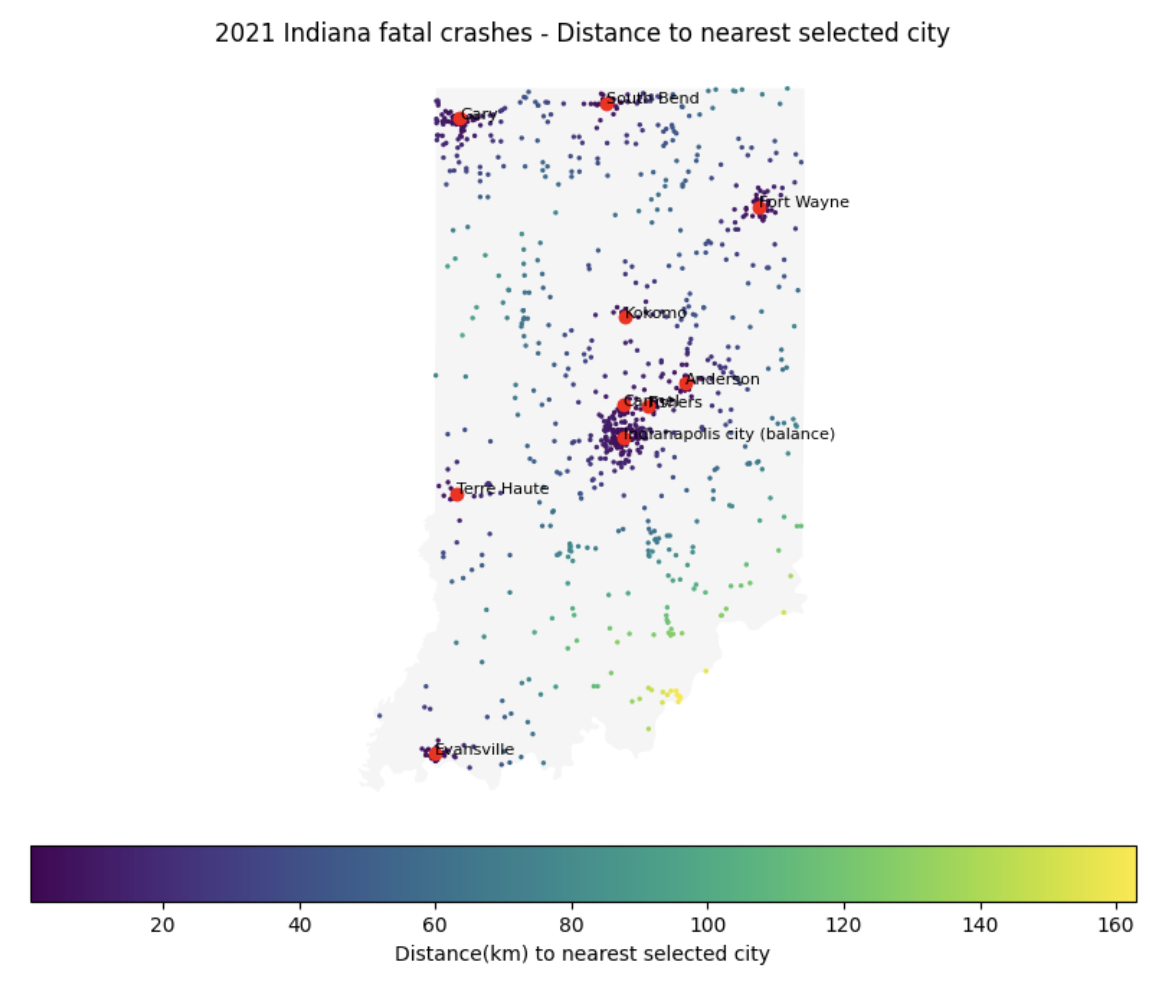
The map conveys multiple information simultaneously: geography, location of the crashes, and distances of crashes (another variable) from certain areas.
-
6a. Code and corresponding documentation, and outputs for all required/mentioned in the question.
-
6b. Write a few sentences describing observations from the PLACES dataset that go beyond what is discussed in the question.
-
6c. Explain the process and reasoning for EPSG conversions. If no conversions were made, or is distance was done on EPSG:4326, would there be problems, and if so what?
-
6d. Centroids were used as reference for distance measurements. Do you think there can be cases where this can be misleading or there could be better methods that can be used?
-
6e. For each visualization, provide your own code documentation/comments, and write a few sentences on what information it conveys, and on your interpretation and analysis.
Submitting your Work
Once you have completed the questions, save your Jupyter notebook. You can then download the notebook and submit it to Gradescope.
-
firstname_lastname_project13.ipynb
|
It is necessary to document your work, with comments about each solution. All of your work needs to be your own work, with citations to any source that you used. Please make sure that your work is your own work, and that any outside sources (people, internet pages, generative AI, etc.) are cited properly in the project template. You must double check your Please take the time to double check your work. See submissions page for instructions on how to double check this. You will not receive full credit if your |