TDM 10200: Project 10 - Visualizations
Project Objectives
Motivation: You can work really hard to come up with quality results from working with data. Presenting your results visually is especially important. This allows you to communicate your findings to others who may not otherwise understand your work. Visualizations not only help communicate results, but also support better interpretation and decision-making.
Context: Plotting in Python can get quite complex and stylistic, but before diving into customization, it is essential to know how to make the basic plots.
Scope: Python, plots, barplots, box and whisker plots
Make sure to read about, and use the template found on the template page, and the important information about project submissions on the submission page.
Dataset
-
/anvil/projects/tdm/data/death_records/DeathRecords.csv
|
If AI is used in any cases, such as for debugging, research, etc., we now require that you submit a link to the entire chat history. For example, if you used ChatGPT, there is an “Share” option in the conversation sidebar. Click on “Create Link” and please add the shareable link as a part of your citation. The project template in the Examples Book now has a “Link to AI Chat History” section; please have this included in all your projects. If you did not use any AI tools, you may write “None”. We allow using AI for learning purposes; however, all submitted materials (code, comments, and explanations) must all be your own work and in your own words. No content or ideas should be directly applied or copy pasted to your projects. Please refer to GenAI page in the example book. Failing to follow these guidelines is considered as academic dishonesty. |
Death Records
Each year, the Centers for Disease Control and Prevention (CDC) publishes the most comprehensive data on mortality in the United States through the National Vital Statistics System. The dataset contains records of all deaths nationwide between 2005 and 2015, with detailed information on causes of death and demographic characteristics of the individuals.
The dataset used for this project contains information from the year 2014 about the mortality data records released by the CDC. This dataset is thorough and contains 38 columns and 2631171 rows of death record data. The columns cover everything from date of death to personal details (age, sex, marital status, etc.) to manner of death and more. Some of the columns may not make a lot of sense and that is OK. Feel free to explore this dataset as much as you would like to gain a better understanding.
Many of the columns only contain encoded values. There are accompanying datasets that will help you understand what is actually being shown. Some examples of these decoder files are provided in Question 1.
Some of the columns from myDF that we will work with include:
-
MonthOfDeath: numerical month of death -
Age: age at time of death -
MaritalStatus: initial representing encoded marital status -
Race: numerical encoded value representing the person’s race
An example of what the decoder files may contain is:
-
Code: numerical value shown in the data, -
Description: actual character meaning represented by theCodevalue.
Questions
|
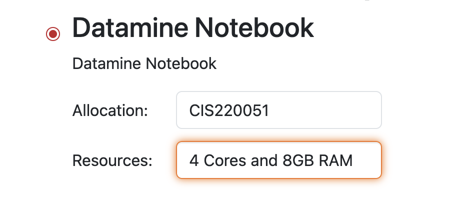
Please use 4 Cores for this project. |
Question 1 (2 points)
Read in the Death Records dataset as myDF from /anvil/projects/tdm/data/death_records/DeathRecords.csv. This dataset is the main source of the death records data, but there are a few different dataset files that go along with myDF that contain the decoder data keys for what the values in some of the columns mean.
Read in the following datasets to ensure correct interpretation of the values from the specific columns Race, and MaritalStatus:
-
/anvil/projects/tdm/data/death_records/Race.csv
-
/anvil/projects/tdm/data/death_records/MaritalStatus.csv
These datasets contain descriptions for what each of the code values of the columns of myDF represent. In the value counts of the column Race in myDF, there are relatively few unique values representing different races. For reference, use the Race.csv dataset to find out what the numerical values of this Race column mean. Also, the number of occurrences of the different values in the Race column varies greatly. Some categories have only a few hundred entries, while others have tens of thousands or more.
Make a plot of these counts to help visualize this. To make a very basic plot in Python, use .plot(). You can specify what kind of plot you want this to be (i.e. .plot(kind='bar')), but that is near the limit of what customization is useful without additional libraries.
import matplotlib.pyplot as pltImport matplotlib, and add a title, x- and y-axis labels. Finally, do plt.show() to display the finished plot.
|
Learn about what kinds of data plots are possible to be made in Python with the helpful datacamp tutorial page. The author shows some different examples of plotting methods, mainly using an example dataset about penguins. For now, it may be helpful to reference the barplot they show. |
1.1 What did you learn about the Race column through the decoder?
1.2 Look at some of the other lines of this dataset that seem like they require a decoder file to be useful. Which of these might be interesting to work with once you have learned what their codes mean?
1.3 Which race had the smallest number of entries?
Question 2 (2 points)
The Race category coded as '1' appears 2241510 times. Compared to other categories with counts such as 700, 4913, or even 13297, this value is disproportionately high, making it difficult to visualize alongside the others on the same scale.
Create a new dataset containing only the entries from the Race column that are not equal to '1':
filtered = myDF[myDF['Race'] != 1]Use .plot() to show this series as either a line plot or a bar plot. Which method do you find more insightful for this data comparison?
Think about your new visualization. How many additional values would you exclude to make the visualization more interpretable? The '2' race values? '3'? More? Less? Try some of these and explain your final decision.
It is almost always a good idea to include as much data as was provided when making a comparison. This can be done, for example, by comparing how many death records of each race there were. But sometimes it is the case that removing data actually helps. If you look at your first plot from Question 1, it is not hard to see that you cannot really tell what is going on with the lower values because the '1' race has extended the upper y-limit so high that everything else is small by comparison.
When you do end up removing the '1' and other values to limit what races are shown, be sure to document this. Write a comment in your notebook about "I removed this value because….." and just explain it a little bit.
When you are finishing these plots, it can also be good to include what values you excluded in the title or labels, like "Death Record Counts by Race (Excluding ….) ". If these plots are just for you, then this gives you a quick reference in some time when you come back and wonder what you plotted. If these plots are for sharing data findings, even better, because these labels help the plot to be interpreted by others who are not in your head.
2.1 How did you make your plot(s) unique to what you know up to this point about plotting?
2.2 How have you ensured your plot(s) are readable for others who might not have as much in-depth knowledge about what you have done here?
2.3 What race(s) did you not include in your final plot, and what is your reasoning that follows this?
Question 3 (2 points)
The MaritalStatus column tracks what relationship stage each person was in at the time of death. Make sure you understand what the letters in this column represent before continuing. Additionally, the values in the Age column range from 1 to 999. Obviously, this 999 is an error code number, not a person who was actually that age. For now, we will keep this value.
The seaborn library is very similar to matplotlib in python. Matplotlib is what is commonly used as default; it gets most things done, and is fairly easy to customize. Seaborn is a higher-level library used for plotting. It is built on matplotlib, and is thus able to provide more options for making appealing visualizations while not over-complicating things.
Use import seaborn as sns!
sns.boxplot is well suited for exploring the relationship between one categorical and one numerical variable. Create a boxplot that shows how the different marital statuses compare to the ages of the people who have died:
sns.boxplot(x='MaritalStatus', y='Age', data=myDF)
plt.title("?????") # customize the title of your plot!!
plt.show()|
Box-and-whisker plots can be confusing to read, even if you are very familiar with what is being shown. Checkout this resource for a bit of help from the page named "How to Read a Box Plot with Outliers". |
It is easy to see where the outliers are in this plot. With the 999 values being so much higher than the other (actual) ages, the rest of the plot gets squished down, so it is not very useful.
Filter out the ages of myDF where they are 999, and save this as cleanDF. With this new cleanDF, make a boxplot to show the reasonable ages and the marital status of the people in the death records.
Take a specific age range (including at least 40 years of ages within the range) from the actual ages of the people who have died, and make a boxplot to show this against the marital statuses.
|
Sometimes the order of the things you are plotting will change places - i.e. The x-axis being plotted as 'M, D, W, S, U' vs when it is plotted as 'D, W, S, M, U'. It is important to make note of this, and set a specific sorted order if needed. |
3.1 Import the seaborn library as sns.
3.2 Compare your boxplot of all of the ages (with the 999 value) vs the boxplot of the actual ages without the 999 value.
3.3 Explain (to your understanding) how the boxplot of the specific age range relates to the boxplot tracking the marital status across all of the ages.
Question 4 (2 points)
Make a boxplot that is very similar to that which you just made, except only for the people whose marital status is "M" (married) OR "W" (widowed). Your plot should have two "boxes", with clearly distinguishable boxes for each marital status.
subset = df[df['col'].isin(['value_1', 'value_2'])]Be sure to continue removing the 999 value from the Age column here. You should have this already done in cleanDF!
For this boxplot, add proper title, axis labels, and colors. Any additional customizations you want to add are welcome.
# make the boxplot
# 'palette' will cause a warning message to appear
# BUT you are able to ignore this
sns.boxplot(x='MaritalStatus', y='Age', data=subset, palette=['color_1', 'color_2'])
# titles for your plot
plt.title("[a very fancy title that describes your plot]")
plt.xlabel("[x-axis label that matches the 'x' data]")
plt.ylabel("[y-axis label that matches the 'y' data]")
# any other customizations
plt.show()
People can die at any age but it is more likely for someone older to be widowed in their death record than it is for a younger person to be. The same is likely true for any status besides single, depending on how young or old of people you are looking at.
So, how do you compare the marital statuses across a certain age? You can plot it.
Take your subset of cleanDF (which should only include the people who were married or widowed). Filter subset to take only the data entries where the peoples' ages were exactly 60. Save this as subset2 to avoid overwriting subset.
Find the value counts of subset2 to see how the marital statuses of the 60-year-olds were distributed between the people that were married vs widowed. Call this my_counts, and put it into a barplot.
|
You can plot this using Pandas, matplotlib, or seaborn! |
4.1 Explain some of what is shown in your Married vs Widowed people (all ages) boxplot to the best of your knowledge.
4.2 Barplot comparing the people who were 60 and were either Married or Widowed. Make at least one other barplot for a different age, and explain what you learned from the two.
4.3 Compare making these barplots using Pandas vs matplotlib vs seaborn. What did you notice?
Question 5 (2 points)
Filter the data of cleanDF to only include the people who are age 60, across all marital statuses. Call this my_first_counts - or whatever name you find fitting.
Do the same for where the people are age 70, and age 80, respectively:
-
my_first_counts - age 60
-
my_second_counts - age 70
-
my_third_counts - age 80
With each subset, get the value counts AND sort by the index. The counts of people of each marital status are different depending on the age, so sorting by the index allows us to keep these three subsets' marital statuses ordered the same.
You have hopefully learned a bit about using Pandas vs matplotlib vs seaborn for when you are wanting to plot.
Plot the value counts of my_first_counts, my_second_counts, and my_third_counts as their own barplot, using whatever method you like. For these barplots, include at least:
-
main title,
-
axis labels,
-
plt.show() (to clean up the plotting space).
5.1 Three barplots; one for the 60-year-olds, the 70-year-olds, and the 80-year-olds.
5.2 How does the distribution of the marital statuses shift across the ages?
5.3 Make a brand new plot. What you show here is completely up to you. Plot something you find interesting from the Death Records dataset, and explain.
Submitting your Work
Once you have completed the questions, save your Jupyter notebook. You can then download the notebook and submit it to Gradescope.
-
firstname_lastname_project10.ipynb
|
It is necessary to document your work, with comments about each solution. All of your work needs to be your own work, with citations to any source that you used. Please make sure that your work is your own work, and that any outside sources (people, internet pages, generative AI, etc.) are cited properly in the project template. You must double check your Please take the time to double check your work. See submission page for instructions on how to double check this. You will not receive full credit if your |