TDM 20200: Project 6 - Introduction to Polars

Before we hop into explaining the major differences between Polars and Pandas, lets start with some basic operations that we are already familiar with in Pandas. They are a little different syntax wise, but overall still fairly intuitive.

The dataset we are using is the NYC Yellow Cab Trip dataset and it is stored as a Parquet file, so just as we would in Pandas, we can import Polars and load in the dataset like so:

So far this is pretty much the exact same as Pandas but we will start seeing some differences once we want to start playing with the data.

Since we are working with a time, location, and money based dataset, lets take a look at some basic statistics of how much each ride costs.

In Pandas, we would do something like this:

In Polars the syntax looks more like this:

The first main difference we notice is that we are not directly indexing onto the dataframe like we do in Pandas, instead we tell Polars what columns we want to use and what operations we want to apply to them. Then we actually apply these operations to the dataset using the .select() method.

These specified operations are called expressions which we will talk more about in a bit. At first, it might seem pointless but this opens the door to a whole new host of optimizations and ways to manipulate your data which is why Polars is so nice!

Here is the link to the documentation which goes over a lot of the functions in Polars.

We already looked at the mean and std of the total_amount column, but lets look at the median and min/max, as well. Check the documentation/look online for the syntax for the specific functions. You can also compare the output of this with the .describe() method in Polars.

Now lets create a new column called trip_duration that calculates the trip duration in minutes (difference between tpep_dropoff_datetime and tpep_pickup_datetime). In Polars, you can subtract datetime columns directly to get a Duration type, then convert it to minutes using .dt.total_minutes().

But we notice that using .select() does not actually change the dataframe, it just returns the resulting column(s) based on your specified expression. To actually see the rest of the dataframe with our new column we should use the .with_columns() method.

If you want to save it to the dataframe you can just reassign it using df = df.with_columns(trip_duration=…​). Now, lets move on to the filter method in Polars. Lets try to filter the dataframe to show only trips where the trip_distance is greater than 5 miles and the passenger_count is greater than 1. We can use the & operator to combine multiple conditions:

Now lets display the shape of the filtered dataframe. The .shape attribute returns a tuple (number_of_rows, number_of_columns):

In Question 1, we briefly mentioned that the operations we specify (like pl.col('total_amount').mean()) are called expressions. Expressions are one of Polars' most powerful and unique features and understanding how they work is crucial to using Polars to its full potential.

So what exactly is an expression? An expression in Polars is a description of a computation - it doesn’t actually execute until you tell it to. Its analogous to a recipe - you are describing what you want to cook and all the ingredients you need, but nothing actually happens until you decide to actually start cooking.

In Pandas, when you write something like df['tip_amount'] / df['total_amount'], it immediately calculates the result. In Polars, when you write pl.col('tip_amount') / pl.col('total_amount'), you are just creating an expression object that describes the computation. Nothing happens until you use it with a method like select(), with_columns(), filter(), or group_by().agg().

Let’s create our first expression. We want to calculate the tip percentage: (tip_amount / total_amount) * 100. We can do this by using the pl.col() function to reference a column named tip_amount and a column named total_amount, then divide tip_amount by total_amount and multiply by 100. Note that pl.col('tip_amount') does not know what the data is nor it is making a reference to our dataset yet. We are simply telling Polars that "there will be a column called tip_amount and a column called total_amount and we want to perform this operation on them".

Notice that this does not return any data - it just creates an expression object.

Now, we can actually apply it to our dataframe using the select() method to compute the result:

If you wanted, you can also create the expression inline:

This will select the column total_amount and then create a new column called tip_percent that is the result of the expression we defined.

Now let’s use with_columns() to add multiple new columns to our original dataframe. We will create:

Now let’s create a more complex expression using conditional logic. Polars has a pl.when().then().otherwise() syntax (which we just saw with the more robust tip calculation) that is similar to "switch" or "case" statements in some languages. We want to categorize trips:

Based on this logic, how we wrote is_high_tip, and what you see in the tip_percent_expr expression, please create trip_category_expr to handle this separation.

Expressions also work with filter(). Here is an example where we can filter based on the number of riders and the overall cost of the trip:

On your own, please find all trips where the tip percentage is greater than 15% AND the total amount is greater than $30. You will need to use the tip_percent_expr expression we created earlier - you can either add it as a column first using with_columns(), or use it directly in the filter expression.

So far, we have been working with Polars in "eager" mode which is when operations execute immediately - similar to how Pandas works. But Polars has another mode called "lazy" mode which is one of its most powerful features. In lazy mode, Polars does not execute operations immediately, rather it builds up a query plan and optimizes it before executing it.

In eager mode, you tell the computer to do things sequentially and immediately, "do this now, now do that, now do this other thing". In lazy mode, you tell Polars "I want to do this, also that, and this other thing" and Polars says "okay, let me think about the best way to do all of that" and then builds up a query plan and optimizes it before executing it.

Since we already have our dataframe loaded in, let’s convert our dataframe to a LazyFrame. We can do this by calling .lazy() on our dataframe:

Notice that when you display a LazyFrame, it does not show the data - it shows the query plan. For a newly created LazyFrame (before any operations), the plan simply shows the table source. This is because nothing has been executed yet.

Now let’s build a lazy query. We want to:

The group_by() method groups rows that have the same value in the specified column(s). Then agg() (short for "aggregate") applies functions like mean(), sum(), count(), etc. to each group. Think of it like SQL’s GROUP BY clause - it creates groups and then computes summary statistics for each group.

Notice how the syntax for this is very similar to eager mode syntax (you can use the same methods like filter(), select(), group_by(), and agg()), except that even if we use lazy_df.filter().select().group_by().agg(), it still does not execute until we explicitly tell it to which we will do momentarily.

Before we do that lets take a look at the graph of the query plan - we see the query plan and the query graph with the operations we specified going from the table, to the filter, to the select, to the group_by, to the agg. But this is the "naive plan" which means that it has not been optimized yet. We can view the optimized plan by calling the show_graph() method which will show the optimized plan:

Now we see the optimized query plan which rearranges some of the operations to be more efficient. Notice that we have 4 columns in the .select() statement and, in the unoptimized plan, we select those 4 columns after the filter. However, Polars looks at the operations and realizes we can select the columns first which will reduce the amount of information we need to filter from so it moves that up first. Also note that the optimized plan only selects 3 columns, not 4.

This is because trip_distance is selected but never used in the aggregation, so Polars eliminates it to reduce memory usage - this is called "projection pushdown" which we will learn more about in Question 5.

Now, to actually execute the query and get results, we need to call .collect():

Now let’s create a more complex lazy query. We want to:

Use the previous example as a guide to create this more complex query. Remember we created a tip_percent_expr expression in the previous question so we can use that here too.

Now let’s compare the performance of eager vs lazy mode. We will do the same operations in both modes and time them:

So far, we have been working with datasets that fit in memory with no issues. But, as we have encountered in previous projects a few times now, what happens when you have a dataset that is too large to fit in memory? This is where Polars' streaming API comes in handy.

Streaming allows Polars to process data in chunks rather than loading everything into memory at once, similar to how you can specify chunksize in Pandas when reading in a dataset.

To use streaming, we first need to create a LazyFrame from the file. Instead of reading the entire dataset into memory first and then converting it to a LazyFrame (i.e. read_parquet().lazy()), we can use scan_parquet() which creates a LazyFrame directly from the file without loading the data into memory:

Notice that printing out the lazy_df shows us the query plan just like it did in Question 3 when we converted our eager DataFrame to a LazyFrame. The key difference is that scan_parquet() never loads the data into memory - it only reads from disk when you call .collect().

Now let’s create a streaming query (same general syntax as the one we worked in Question 3). We want to:

Once you have written the query, to execute it with streaming, we use .collect(engine='streaming'). Without the engine='streaming' parameter, Polars would try to load all the data into memory first (if using read_parquet().lazy()) or process the dataset all at once, which could fail for very large datasets:

Let’s compare streaming vs non-streaming performance. We will execute the same query both ways and time them:

Now let’s create a more complex streaming query. We want to find the average tip percentage by hour of day:

Throughout this project, we have mentioned that Polars is faster than Pandas, but we have not really explored why it is faster besides "optimization". In this final question, we will dive into the underlying technology that makes Polars so fast: Apache Arrow’s Columnar Format (ACF) and Polars' query engine.

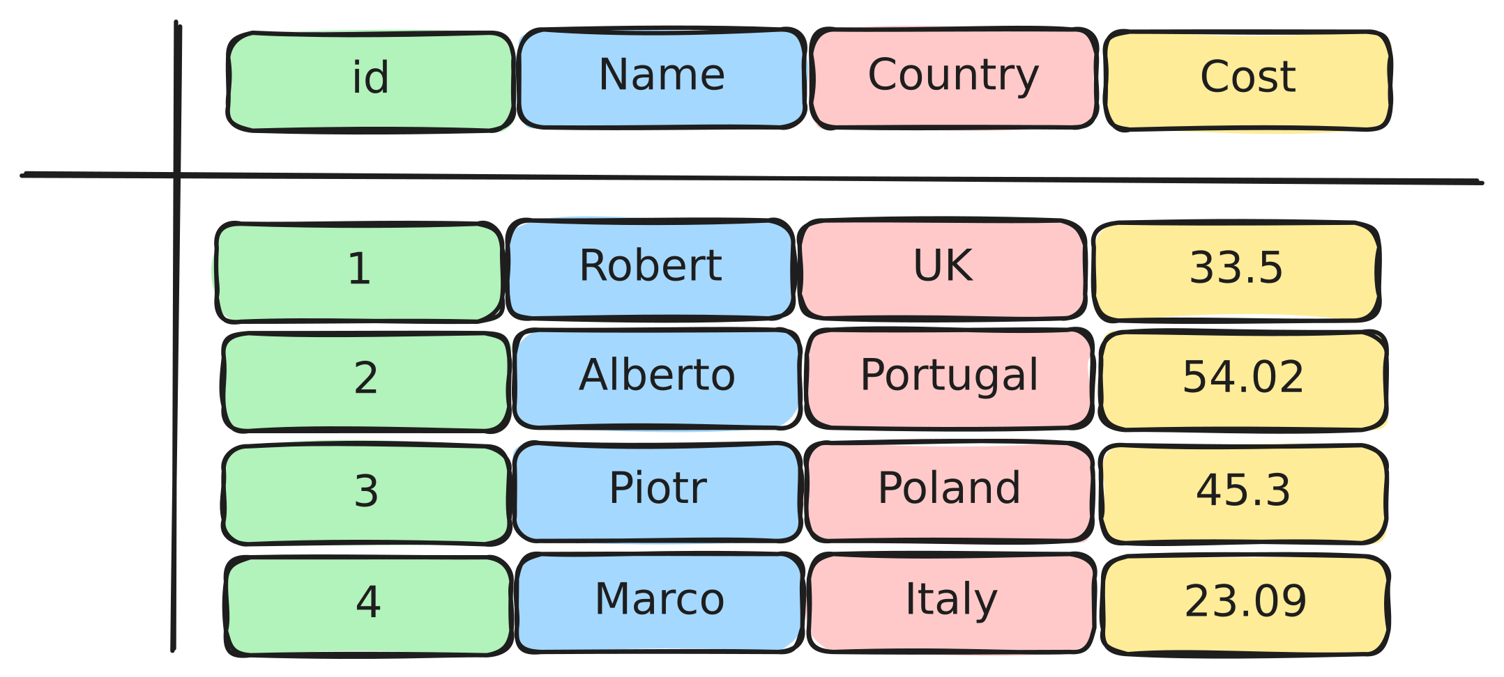
Polars is built on Apache Arrow, which uses a columnar memory format. This is fundamentally different from how Pandas stores data. First lets take a look at a diagram of an example dataframe:

Pandas takes this dataframe and stores it row-by-row (like a spreadsheet) in memory which looks like this:

However, in Polars (using Arrow), data is stored column-by-column. This might seem like a small difference, but it has huge implications for performance.

The data for each column is stored in contiguous memory blocks which means that the data for each column is stored together in order in memory.

Let’s first explore the Arrow Columnar Format. Load your dataframe and check its memory usage:

In Question 3, we saw that lazy evaluation allows Polars to see your entire query and optimize it before executing. Now let’s explore advanced query optimization in more detail. We will create a lazy query with multiple operations and see the specific optimizations Polars applies:

Now let’s see the optimized query plan:

Look at the optimized query plan and explain in a comment what optimizations you see. Common optimizations include:

You may also notice that Polars can combine or merge multiple operations together (like combining multiple with_columns() calls into one), which is part of its general query optimization.

Now let’s create a complex transformation and compare it to how you might do it in Pandas. We want to calculate percentage breakdowns for all cost columns:

Now let’s see the equivalent Pandas version:

Also note the difference between using the eager and lazy dataframe versions (df.select() vs lazy_df.select().collect()) for this operation compared to Pandas. The lazy version will not crash the kernel as easily because it is not loading all the data into memory at once, but in some cases it may process the data as slow or slower than Pandas. The eager version however, since it can parallelize all the operations in memory, should be much faster than Pandas.

Now let’s explore parallelization a little more. The key insight is that Polars can process different columns in parallel because they are stored separately in memory.

Let’s create a query that performs multiple aggregations on different columns:

In this query, we are computing multiple aggregations on different columns. Because these columns are stored separately in memory (columnar format), Polars can process these aggregations simultaneously on different CPU cores. This is the parallelization.

In row-based storage (like Pandas), this is much harder because all the data for a row is stored together, making it difficult to process different columns independently and in parallel.

This is a more complex query that might crash the notebook when trying to run .collect() on it. This can happen with large datasets when Polars tries to parallelize operations so we should use .collect(engine='streaming') instead like we mentioned in the previous questions to circumvent this issue!