TDM 30100: Project 12 - Random Forest - Predicting Prescribers
Project Objectives
In this project, you will build a decision tree and random forest model to predict whether prescribers will prescribe Semaglutide.
Dataset(s)
-
/anvil/projects/tdm/data/CMS/RandomForest_F25/X_train_rf -
/anvil/projects/tdm/data/CMS/RandomForest_F25/X_val_rf -
/anvil/projects/tdm/data/CMS/RandomForest_F25/X_test_rf -
/anvil/projects/tdm/data/CMS/RandomForest_F25/y_train_rf -
/anvil/projects/tdm/data/CMS/RandomForest_F25/y_val_rf -
/anvil/projects/tdm/data/CMS/RandomForest_F25/y_test_rf
|
This project picks up where you left off with our recent logistic regression seminar project. You already did the hard work which was building a model, interpreting the results, and prepping the data through processing and scaling to help the model perform better. Now that the data is ready to go, we will shift our focus to building and comparing a decision tree and a random forest model. We have provided the pre-processed datasets (X_train_rf, y_train_rf, etc.) so you can dive right into modeling without worrying about cleaning the data again. |
|
If AI is used in any cases, such as for debugging, research, etc., we now require that you submit a link to the entire chat history. For example, if you used ChatGPT, there is an “Share” option in the conversation sidebar. Click on “Create Link” and please add the shareable link as a part of your citation. The project template in the Examples Book now has a “Link to AI Chat History” section; please have this included in all your projects. If you did not use any AI tools, you may write “None”. We allow using AI for learning purposes; however, all submitted materials (code, comments, and explanations) must all be your own work and in your own words. No content or ideas should be directly applied or copy pasted to your projects. Please refer to the-examples-book.com/projects/fall2025/syllabus#guidance-on-generative-ai. Failing to follow these guidelines is considered as academic dishonesty. |
About the Data
This dataset comes from CMS and includes prescription-level records for diabetes medications. Each row represents a unique prescriber writing a prescription for a specific brand-name drug. Among these drugs is Semaglutide, the drug name behind Ozempic, a medication approved for type 2 diabetes. The original 2023 data comes from the link: Centers for Medicare and Medicaid Services (CMS) dataset.
|
Use 4 cores for this project. |
Variables in the Data
Below are the columns you will be working with in this project. Remember, these were the selected features in the final model of the logistic regression project.
| Column Name | Description |
|---|---|
|
Calculated as |
|
Indicator variable (0 or 1) for whether the prescriber falls under the Primary Care category. |
|
Indicator variable (0 or 1) for prescribers grouped into Gastroenterology, Renal, or Rheumatology specialties. |
|
Total number of days of medication supplied across all claims for the prescriber-drug combination (scaled). |
|
Indicator variable (0 or 1) for prescribers in the Endocrinology specialty. |
|
Indicator variable (0 or 1) for prescribers grouped under Neurology or Psychiatry. |
|
Indicator variable (0 or 1) for cases where the prescriber specialty was missing or ungrouped. |
|
Indicator variable (0 or 1) for prescribers whose specialty is grouped under Surgery. |
|
Indicator variable (0 or 1) for prescribers that don’t fall into predefined specialty groups and are labeled as “Other.” |
|
Indicator variable (0 or 1) for prescribers in Obstetrics, Gynecology, or other Women’s Health fields. |
|
Indicator variable (0 or 1) identifying prescribers located in the Southern U.S. region. |
In this project, you will first train a decision tree to understand the logic behind tree splits and predictions. Then, you will train a random forest to improve accuracy and explore how ensemble models work. We will review decision trees and go over how random forest work under the good. Along the way, you will evaluate each model’s performance and think critically about model confidence and real world use cases.
What is an Ensemble Model?
Imagine you are choosing a movie. Instead of asking just one friend, you ask five friends and go with what most of them recommend. That’s how ensemble models work: they combine the predictions of multiple models to make a final decision.
Why Use an Ensemble?
A single model (like a decision tree) might make mistakes or overfit the data. But when we combine multiple models, we can get:
-
More accurate predictions,
-
More reliable results.
Why Use These Models in Healthcare Data?
In healthcare and pharmaceutical analytics, we often want to:
-
Predict outcomes (e.g., Will a provider prescribe a new drug?),
-
Understand feature importance (e.g., What specialties are more likely to prescribe it?),
-
Balance performance with interpretability.
Decision trees and random forests are good tools for this kind of work. You can get insight from a simple tree and then scale up to a more powerful random forest for better predictions.
Questions
Question 1 - Understanding the Data (2 points)
In the previous logistic regression project, you learned how to build an interpretable model to identify important features associated with Semaglutide prescriptions.
|
Remember, in the recent logistic regression project we split the data into different subsets to help build and evaluate the model. We also pre-processed each dataset, standardized numeric features and one-hot encoded categorical variables. |
Let review what each subset is again as we will be utilizing these data splits in this project:
| Subset | X (Predictors) | y (Target Labels) |
|---|---|---|
Training |
|
|
Validation |
|
|
Test |
|
|
1a. Read in each dataset using the code below and then print how many total observations are in your training, validation, and test datasets.
import pandas as pd

X_train_rf = pd.read_csv("/anvil/projects/tdm/data/CMS/RandomForest_F25/X_train_rf.csv")
X_val_rf = pd.read_csv("/anvil/projects/tdm/data/CMS/RandomForest_F25/X_val_rf.csv")
X_test_rf = pd.read_csv("/anvil/projects/tdm/data/CMS/RandomForest_F25/X_test_rf.csv")

y_train_rf = pd.read_csv("/anvil/projects/tdm/data/CMS/RandomForest_F25/y_train_rf.csv").values.ravel()
y_val_rf = pd.read_csv("/anvil/projects/tdm/data/CMS/RandomForest_F25/y_val_rf.csv").values.ravel()
y_test_rf = pd.read_csv("/anvil/projects/tdm/data/CMS/RandomForest_F25/y_test_rf.csv").values.ravel()
1b. Calculate and print the proportion of records where Semaglutide_drug = 0 and Semaglutide_drug = 1 in each dataset (y_train_rf, y_val_rf, and y_test_rf).
Hint:
You can use pd.Series(DF).value_counts(normalize=True)).
1c. Write 1-2 sentences to comment on class balance. Would you consider this dataset imbalanced in terms of proportions of 0’s and 1’s? Why or why not?
Question 2 - Decision Trees (2 points)
Review Decision Trees
Decision trees are a popular tool for making predictions in machine learning. They can be used for both regression (predicting numbers) and classification (predicting categories). In this project, we’re focused on classification specifically, predicting whether a prescriber will prescribe Semaglutide (yes or no).
Review: What Is a Decision Tree?
You can think of a decision tree like a flowchart:
-
At each step (called a node), the model asks a yes/no question about one of the features (like
Cost_per_claimorTotal_Day_Supply). -
Depending on the answer, the data follows one of two branches.
-
This continues until it reaches a leaf or terminal node, where a prediction is made.
The goal is to keep splitting the data into smaller and smaller groups that are more pure which means most observations in each group belong to the same class.
How Does the Model Make Splits?
Decision trees are built using a process called recursive binary splitting:
-
The model starts with the entire dataset.
-
It looks through all possible features and cut-off values and picks the one that best separates the data into groups with different outcomes.
-
It repeats this within each subgroup, splitting again and again until it reaches a stopping point like a maximum tree depth or a minimum number of observations per group.
Each group that results from a split is called a region, and each split is chosen to increase node purity.
What Does the Tree Represent?
The tree divides the dataset into boxes (or regions) based on the feature values. For example:
If Cost_per_claim < 200:
    Predict Not Semaglutide
Else:
    If Total_Day_Supply > 180:
        Predict Semaglutide
    Else:
        Predict Not Semaglutide
We start with decision trees in this project because they are easy to interpret and help us understand how the model is making predictions. Once we understand and review them, we will move on to random forests, which build on decision trees to create more complex and accurate models.
How to Interpret a Decision Tree
Each path from the top (the root node) to the bottom (a leaf node) represents a sequence of decisions that leads to a final predicted class.
Basic Structure
-
Nodes: Each box in the tree is called a node. It includes:
-
A splitting rule (e.g.,
feature ⇐ threshold) -
The gini impurity, which measures how mixed the classes are at that node. A gini of 0 means the node is pure (only one class), while a gini close to 0.5 means it’s a 50/50 mix.
-
The number of samples that reached this node.
-
The value, which shows how many records belong to each class at that node.
-
The predicted class, which is the majority class at that node.
-
-
Branches: These are the lines that connect the nodes. Each branch represents the outcome of a condition—if the condition is true, the model moves to the left; if false, it moves to the right.
-
Leaf Nodes: These are the final nodes at the bottom of the tree. They represent the model’s predicted class for any data point that ends up there.
How to Read It
To interpret a decision tree:
-
Start at the top and follow the branches based on the conditions.
-
At each node, decide whether the condition is true or false.
-
Continue until you reach a leaf node, which gives the predicted class.
What to Pay Attention To
-
Which features are used for splitting? Features near the top of the tree are usually more influential.
-
What do the gini values tell you? The lower the gini, the more confident the model is in that node’s classification.
-
What are the class distributions? Look at the
valuefield to see how many examples from each class ended up in the node. This helps you judge the strength of the prediction.
Why This Matters
Interpreting a decision tree helps you:
-
Understand how the model is making decisions.
-
Identify important patterns in the data.
-
Gain insight into which features are most useful for predicting the outcome.
Model Performance - Review
Confusion Matrix
This is a 2x2 table that shows how many predictions your model got right and wrong for each class.
| Predicted: 0 | Predicted: 1 | Total (Actual) | |
|---|---|---|---|
Actual: 0 |
True Negative (TN) |
False Positive (FP) |
TN + FP |
Actual: 1 |
False Negative (FN) |
True Positive (TP) |
FN + TP |
Classification Report
This includes:
-
Precision: Of all predicted Semaglutide prescribers, how many actually prescribed it?
-
Recall: Of all actual Semaglutide prescribers, how many were correctly predicted?
-
F1-score: Mean of precision and recall
-
Support: How many examples belong to each class.
AUC (Area Under the ROC Curve)
-
Measures the model’s ability to separate the classes based on predicted probabilities.
-
Ranges from 0.5 (random guessing) to 1.0 (perfect prediction).
-
AUC is threshold-independent, meaning it looks at the model’s performance across all thresholds.
For a deeper explanation of precision, recall, f1-score, confusion matrices, and AUC, see the official scikit-learn documentation:
Visual Explanation of Decision Trees
Here are some great videos to help you visually understand and review how decision trees work!:
2a. Use the code below to fit a DecisionTreeClassifier on the training data using class_weight='balanced', max_depth = 2, and random_state=42. Then, on your own, print the number of leaves along with the tree depth and explain what the depth and leaves represent in the context of a decision tree in 1–2 sentences.
Note: Use the code below to answer 2a. Make sure to fill in the blank spaces in dt_model, print the number of leaves along with the tree depth, and then explain depth and leaves in the context of decision trees in 1-2 sentences.
import pandas as pd
from sklearn.tree import DecisionTreeClassifier
from sklearn.metrics import classification_report, confusion_matrix, roc_auc_score
dt_model = DecisionTreeClassifier(class_weight='____', max_depth=___, random_state=____) # For YOU to fill in
dt_model.fit(X_train_rf, y_train_rf)
print(f"Tree depth: {dt_model.get_depth()}")
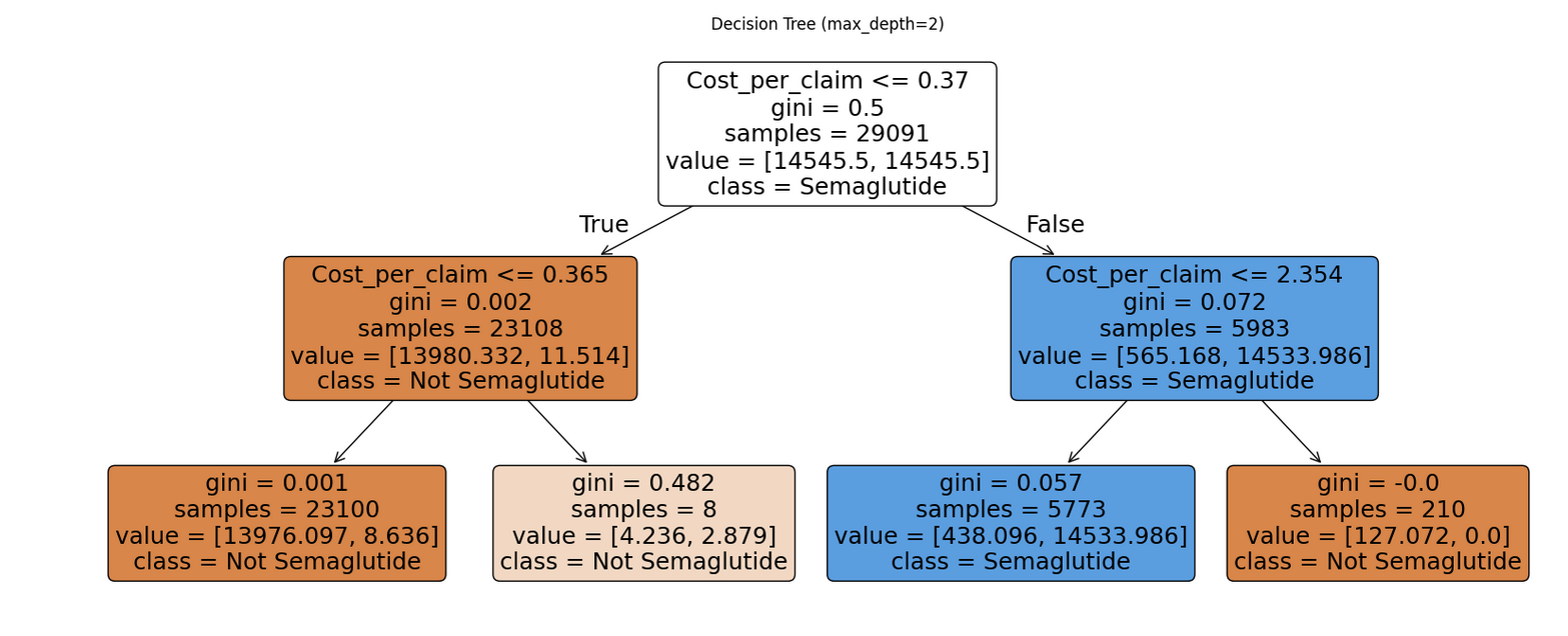
print(f"Number of leaves: {dt_model.get_n_leaves()}")2b. Using the code below, visualize the decision tree using plot_tree() from sklearn.tree on the training data.
Note: The code structure below is mostly complete. Your task is to fill in the missing parts: provide the correct class labels and give a title to the plot. To determine the correct labels, refer back to the order of your results from Question 1b, where you explored the distribution of Semaglutide prescriptions.
import pandas as pd
from sklearn.tree import DecisionTreeClassifier, plot_tree
from sklearn.metrics import classification_report, confusion_matrix, roc_auc_score
import matplotlib.pyplot as plt

plt.figure(figsize=(20, 8))
plot_tree(dt_model,
          feature_names=X_train_rf.columns,
          class_names=["....", "....."], # For YOU to fill in
          filled=True,
          rounded=True)
plt.title(".......") # For YOU to fill in
plt.show()
2c. Run the code below to evaluate the model on the test set using a confusion matrix and the classification report. Then in 1-2 sentences write about the model’s performance.
Note: Your task is to run the code below and then interpret the results in your own words using 1-2 sentences.
from sklearn.metrics import confusion_matrix, classification_report, roc_auc_score

y_test_pred_dt = dt_model.predict(X_test_rf)
y_test_proba_dt = dt_model.predict_proba(X_test_rf)[:, 1]
auc_dt_test = roc_auc_score(y_test_rf, y_test_proba_dt)

print("Decision Tree Performance on Test Set:")
print("Confusion Matrix:")
print(confusion_matrix(y_test_rf, y_test_pred_dt))
print("\nClassification Report:")
print(classification_report(y_test_rf, y_test_pred_dt))
print(f"AUC: {round(auc_dt_test, 4)}")
2d. Look at the first split in your decision tree and write 1–2 sentences explaining what feature is used, what the condition is and what this tells you about the model.
Question 3 - Build and Evaluate a Random Forest Model (2 points)
Why Random Forests?
"Decision trees have one aspect that prevents them from being the ideal tool for predictive learning — namely inaccuracy." — Elements of Statistical Learning
Random forests improve this by combining bootstrapped datasets and random predictor selection leading to diverse trees and better performance.
How it Works
Step 1: Create a Bootstrapped Dataset
We start with a dataset like this:
| Tot_Day_Suply | Cost_per_claim | Prscrbr_Type_PrimaryCare | Region_South | Semaglutide |
|---|---|---|---|---|
0.856944 |
-0.312060 |
1 |
1 |
0 |
0.831318 |
-0.309074 |
1 |
0 |
0 |
1.132426 |
-0.315260 |
1 |
1 |
0 |
-0.434619 |
0.870000 |
0 |
0 |
1 |
0.380723 |
-0.311051 |
1 |
0 |
0 |
We create a bootstrapped dataset by sampling rows with replacement:
| Tot_Day_Suply | Cost_per_claim | Prscrbr_Type_PrimaryCare | Region_South | Semaglutide |
|---|---|---|---|---|
1.132426 |
-0.315260 |
1 |
1 |
0 |
-0.434619 |
0.870000 |
0 |
0 |
1 |
0.831318 |
-0.309074 |
1 |
0 |
0 |
1.132426 |
-0.315260 |
1 |
1 |
0 |
Step 2: Build a Tree Using Random Predictors
When splitting the data:
-
The tree selects a random subset of predictors (e.g. 2 or 3 out of 11)
-
Suppose we randomly pick:
Cost_per_claim, andPrscrbr_Type_PrimaryCare -
The tree uses the best of those to split.
Each node repeats this process with a new random subset.
Step 3: Repeat to Build a Forest
Repeat:
-
Create new bootstrapped data
-
Build new tree using random predictors
-
Repeat hundreds of times
The result: a forest of trees, each slightly different! This diversity helps reduce variance and avoid overfitting.
After running the data down all trees in the random forest, we see which option received more votes. In this case "1" received more votes, so we will conclude the prescriber did prescribe semaglutide.
Step 4: Estimate Accuracy Using Out-of-Bag (OOB) Error
How do we know if the random forest is any good? Some rows are not included in each bootstrapped sample, these are called Out-of-Bag samples.
We use them like test data:
-
For each row, run it through all trees that didn’t train on it.
-
Each tree votes:
Semaglutide = 0or1 -
Take the majority vote and compare to the true label
Row = 2220
True label = 1
Out-of-Bag (OOB) predictions: 1, 1, 0, 1
→ majority vote = 1
→ Correct!
Repeat for every row.
Then we run the out-of-bag sample through all the other trees that were built without it. Since the label with the most votes wins, it is the label that we assign the out of bag sample. We then to the same thing for all the other out of bag samples for all the other trees.
Ultimately, we can measure how accurate our random forest model is by the proportion of out of bag samples that were correctly classifified by the random forest. The proportion of the Out-of-bag samples that were incorrectly classified is the "Out-of-Bag" error.
Why This Works
By making each tree slightly different through both bootstrapping and random predictor selection, random forests produce more reliable predictions.
How Predictions Are Made
-
Classification: Each tree votes for a class label. The final prediction is the majority vote.
-
Regression: Each tree gives a numeric prediction. The final prediction is the average.
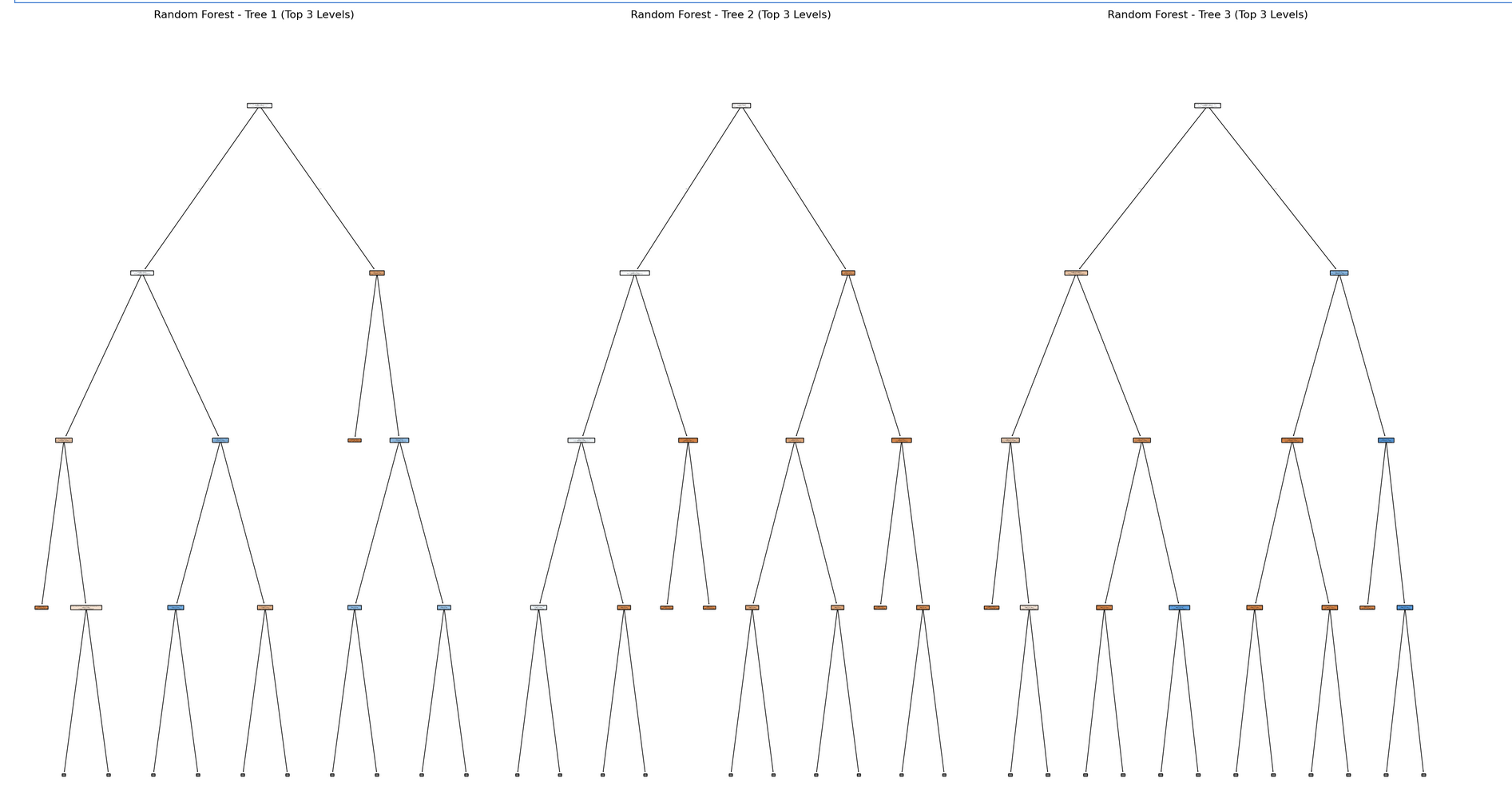
Visualize a FEW Trees (3) from the Random Forest Model
Important Terminology
| Term | Definition |
|---|---|
Random Forest |
An ensemble method that builds many decision trees on random subsets of the data and predictors, then combines them by averaging (regression) or voting (classification). |
Decision Tree |
A model that makes decisions by splitting data into branches based on conditions on predictor variables. |
Bootstrapping |
Sampling from the original dataset with replacement to create a new dataset the same size. |
Bagging |
Short for bootstrap aggregating: training multiple models on bootstrapped data and averaging the results. |
Out-of-Bag (OOB) Sample |
Data points that were not selected in a given bootstrap sample, used like a built-in validation set. |
Out of Bag (OOB) Error |
An estimate of the model’s prediction error, calculated using only the OOB predictions for each observation. |
m |
Number of predictor variables randomly selected at each split in a tree. |
Ensemble |
A group of models combined to produce a stronger overall prediction. |
Majority Vote |
In classification, the final predicted class is the one that most trees predict. |
What Happens When You Plot a Random Forest
When you try to plot a Random Forest, you’ll notice something right away: there are a lot of trees!
This is because a Random Forest is not just one tree it’s an ensemble of many decision trees (often 100, 200, or even more). Each tree is trained on a slightly different version of the data and makes its own predictions.
Why does the plot have so many branches?
Take a look at the image below it’s a visualization of just ONE of the trees from a Random Forest. And even that can be pretty big (the image below is just a small section of the entire tree)!
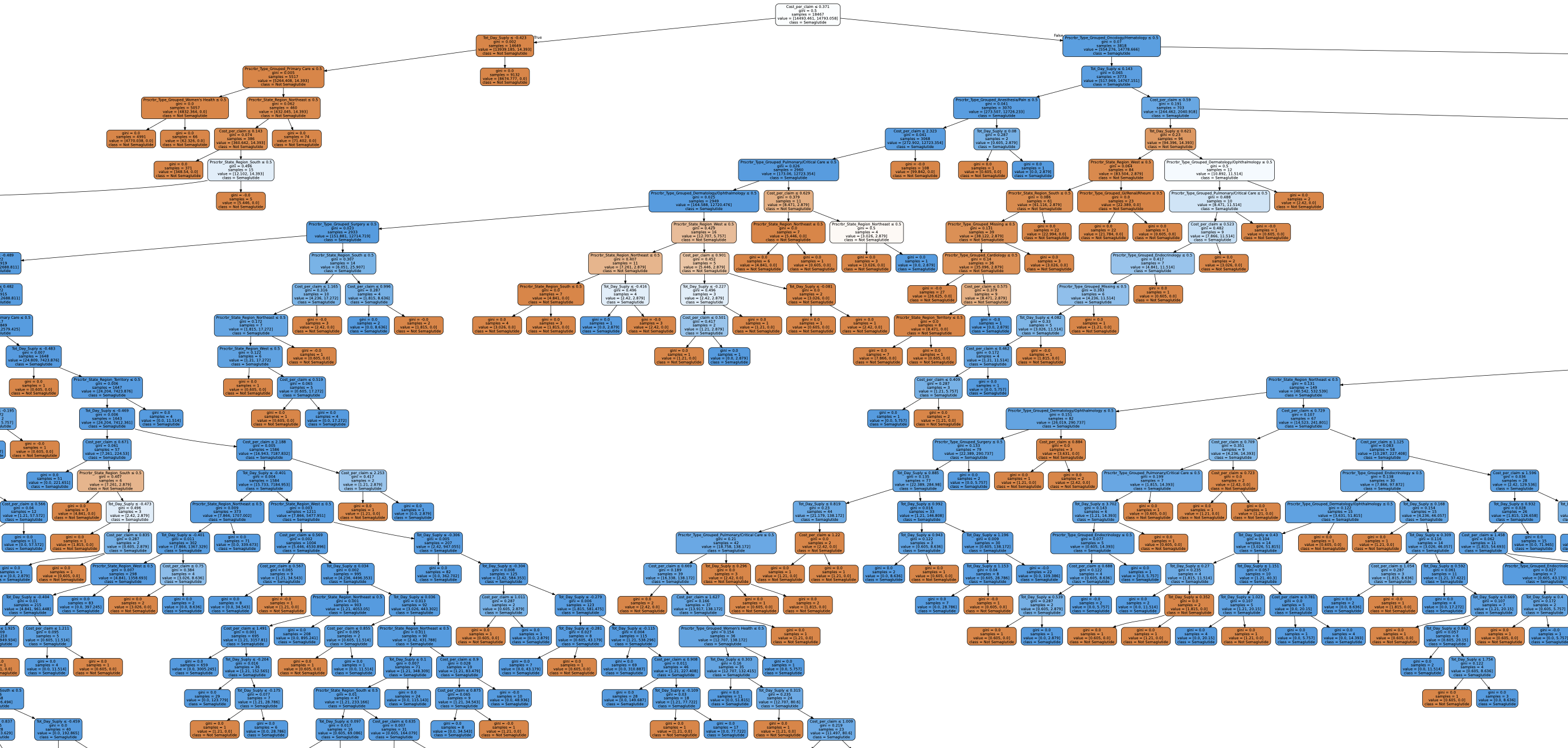
Now imagine 100 of these trees! Plotting the entire forest at once have many trees and be difficult to use for interpretation.
So What Can You Do Instead?
Instead of plotting the entire forest, we usually:
-
Plot just one representative tree from the forest.
-
Look at feature importance to understand which variables matter most.
-
Use metrics and visualizations (like confusion matrices, ROC curves, and precision scores) to evaluate model performance.
Key Takeaway
Random Forests are powerful because they combine many trees, but this also makes them less interpretable than a single decision tree. That’s why we often visualize just parts of the model rather than the whole forest.
Summary
We built a tree …..
-
Using a bootstrapped dataset.
-
Only considered a random subset of variables at each step.
-
Keep repeating! Make a new bootstrapped dataset and build a tree considering a subset of variables at each step.
-
Ideally, you do this hundreds of times.
-
Use a bootstrapped sample and consider only a subset of variables at each step results in a wide variety of trees.
-
This variety is what makes random forest more effective than individual decision trees!
Visual Explanation of Random Forest
Here are some great videos to help you visually understand and review how Random Forest work!:
3a. Use the code below to fit a RandomForestClassifier on the training data using class_weight='balanced', random_state=42 After fitting the model, write 1–2 sentences explaining how Random Forest models work and how they differ from a single decision tree.
Note: Most of the code has been provided for you below. Make sure to fill in the missing pieces.
from sklearn.ensemble import RandomForestClassifier
from sklearn.metrics import roc_auc_score, classification_report, confusion_matrix
import matplotlib.pyplot as plt
import pandas as pd
import numpy as np

rf_model = RandomForestClassifier(class_weight='______', random_state=_____) # For YOU to fill in

rf_model.fit(X_train_rf, y_train_rf)
3b. Print the AUC on X_test_rf by running the code below and then write 1-2 sentences evaluating the performance.
Note: The code to print the AUC and confusion matrix for the test set has been provided. We ask that you try to understand and interpret the results in 1-2 sentences.
y_test_pred_rf = rf_model.predict(X_test_rf)
y_test_proba_rf = rf_model.predict_proba(X_test_rf)[:, 1]
auc_rf_test = roc_auc_score(y_test_rf, y_test_proba_rf)

print("\nRandom Forest Performance on Test Set:")
print("Confusion Matrix:")
print(confusion_matrix(y_test_rf, y_test_pred_rf))
print("\nClassification Report:")
print(classification_report(y_test_rf, y_test_pred_rf))
print(f"AUC: {round(auc_rf_test, 4)}")
3c. Compare the Random Forest to your Decision Tree results from 2c. Write 1–2 sentences describing how the performance metrics (e.g., AUC, precision) changed and why that might be expected.
3d. Write 2-3 sentences, in your own words, on the role bagging and bootstrapping plays in building a random forest model.
Question 4 - Feature Importance (2 points)
Interpreting the Model
Building a model that makes good predictions is only part of the story we also want to understand how the model makes decisions.
In real world applications like healthcare, finance, and criminal justice, being able to explain your model is important. Doctors, patients, regulators, and other stakeholders need to know:
-
What factors most influence the prediction?
-
Are those factors reasonable and ethical?
-
Can we justify the model’s recommendations?
Random Forests are more complex than individual decision trees, but we can still interpret them using tools like:
-
Feature Importance: Which variables had the biggest impact on the model’s predictions?
-
Class Proportions for Key Features: What patterns do we see between important features and the target outcome?
In the questions that follow, you will practice:
-
Visualizing which features were most important to your model,
-
Exploring how one of those features differs across your target classes,
-
Reflecting on whether those patterns make sense in the context of your data and objective.
4a. Identify and visualize the top 10 most important predictors from X_train_rf in your random forest model using the code below.
Note: Make sure to fill in the missing parts to:
-
Title and label the plot
import pandas as pd
import matplotlib.pyplot as plt

# Step 1: Extract feature importances from the model
feature_importances = pd.Series(rf_model.feature_importances_, index=X_train_rf.columns)

# Step 2: Get the top 10 most important features
top10_features = feature_importances.sort_values(ascending=False).head(10)

# Step 3: Plot the top 10 features
plt.figure(figsize=(10, 6))
top10_features.plot(kind='barh')
plt.gca().invert_yaxis()
plt.xlabel("______") # For YOU to fill in
plt.title("____") # For YOU to fill in
plt.tight_layout()
plt.show()
4b. Calculate the proportion of primary care prescribers within each class (Semaglutide = 0 and Semaglutide = 1), and then write 1-2 sentences on your interpretation of the results.
Note: Complete the missing parts of the code below (marked with # For YOU to fill in). Think about what variable represents the prescriber type primary care and fill in the quotations with the name of that variable. Then interpret the results.
print(X_train_rf.columns)

# Choose a binary feature from the top 10
binary_feature = "____________" # For YOU to fill in

# Combine features with target
df = X_train_rf.copy()
df["target"] = y_train_rf

# Group by target and compute proportion with value 1
proportions = df.groupby("target")[binary_feature].mean()

print(proportions)
4c. Write 1-2 sentences to explain what the top 3 most important features are capturing in terms of prescribers of Semaglutide and whether the findings seem expected or unexpected.
Question 5 - Confidence In The Model (2 points)
Machine learning models like random forests do not just give you a predicted class they also estimate how confident they are by outputting a predicted probability. By default, we often classify cases as 1 (e.g., "will prescribe Semaglutide") if the probability is greater than or equal to 0.5. But in practice, you might want to adjust this threshold depending on the business or healthcare context.
For example:
A higher threshold (e.g., 0.9) may reduce false positives but miss potential opportunities. A lower threshold (e.g., 0.3) may catch more positives, but with less certainty.
This question helps you explore how confident your model is and why thresholds matter.
5a. Use the predict_proba() method to check how confident the model is in its predictions. Randomly select five prescribers from the test set X_test_rf. For each one, print the predicted probability that they will prescribe Semaglutide, the actual class label (0 or 1), and the predicted class based on a 0.5 threshold.
Note: Use the code provided code below and make sure to fill in the test data frame X_test_rf in which you will be selecting the random 5 samples from.
import numpy as np

# Pick 5 random test examples
random_indices = np.random.choice(len(________), 5, replace=False) # For YOU to fill in

for i in random_indices:
    prob = rf_model.predict_proba(X_test_rf.iloc[[i]])[:, 1][0]
    pred_class = int(prob >= 0.5)
    actual_class = y_test_rf[i]

    print(f"Prescriber {i}:")
    print(f"  Predicted probability of Semaglutide: {round(prob, 3)}")
    print(f"  Final prediction: {pred_class}")
    print(f"  Actual label: {actual_class}\n")
5b. Write 1–2 sentences describing how knowing the probability (not just the predicted label) of a prescriber prescribing semaglutide might be useful in a real-world healthcare or pharmaceutical setting.
5c. Use the code below to find out how many prescribers in the test set were predicted with high confidence (model gave them a probability greater than 0.9 of prescribing Semaglutide).
Note: Use the code provided below. Make sure to fill in the line that identifies the threshold for high-confidence predictions.
# Get predicted probabilities for class 1 (Semaglutide)
probs = rf_model.predict_proba(X_test_rf)[:, 1]

threshold = _____ # For YOU to fill in
preds = (probs >= threshold).astype(int)
high_confidence = probs >= threshold

# Check how many were correct
correct = (preds == y_test_rf) & high_confidence
incorrect = (preds != y_test_rf) & high_confidence

print(f"Total high-confidence predictions (>0.9): {high_confidence.sum()}")
print(f"Correct high-confidence predictions: {correct.sum()}")
print(f"Incorrect high-confidence predictions: {incorrect.sum()}")
5d. Write 1–2 sentences interpreting what this tells you about your model’s confidence and how that could be useful in a real-world healthcare or business setting.
References
Some explanations, examples, and terminology presented in this section were adapted from the following sources for educational purposes:
-
James, G., Witten, D., Hastie, T., Tibshirani, R., & Taylor, J. (2023). An Introduction to Statistical Learning: with Applications in Python. Springer Texts in Statistics. Springer.
-
Scikit-learn Documentation. (2024). Scikit-learn: Classification Metrics
-
Starmer, J. (2020). Random Forests Part 1 – Building, Using and Evaluating. StatQuest with Josh Starmer. www.youtube.com/watch?v=J4Wdy0Wc_xQ
-
Starmer, J. (2020). Decision Tree Classification Clearly Explained!. StatQuest with Josh Starmer. Decision Tree Classification Clearly Explained!
-
Starmer, J. (2020). Decision and Classification Trees, Clearly Explained!!!. StatQuest with Josh Starmer. Decision and Classification Trees, Clearly Explained!!! – StatQuest
-
Art of the Problem. (2020). Visual Guide to Random Forests
Submitting your Work
Once you have completed the questions, save your Jupyter notebook. You can then download the notebook and submit it to Gradescope.
-
firstname_lastname_project12.ipynb
|
You must double check your You will not receive full credit if your |