TDM 40200 Project 7 - Signal Processing

Project Objectives

This project focuses on some fundamental signal processing and audio analysis concepts. We begin with sine waves which are basic building blocks of sound, then we will explore Fourier transforms and related concepts and how we can implement these concepts in Python. Using various libraries (ex. Librosa, NumPy) we will also be computing and visualizing frequency spectra of both notes and real audio recordings using the dataset mentioned below.

Dynamic Time Warping is a method for measuring similarities between two given sequences that can have differences in characteristics such as tempo. We will explore some basic concepts in this algorithm, and understand how it can be applied.

Learning Objectives

Generate and visualize sine waves, and explore sampling and mathematical transformations related to time and frequency domains
Understand and apply Fourier transforms
Visualize audio signals
Manipulate audio
Understand and apply Dynamic Time Warping

Dataset

/anvil/projects/tdm/data/ravdess
RAVDESS (Ryerson Audio-Visual Database of Emotional Speech and Song): a validated database of emotional speech and song. Please refer to the ravdess page in the example book for more info.
Also, the same data set was used last week in Project 6.

If AI is used in any cases, such as for debugging, research, etc., we now require that you submit a link to the entire chat history. For example, if you used ChatGPT, there is an “Share” option in the conversation sidebar. Click on “Create Link” and please add the shareable link as a part of your citation.

The project template in the Examples Book now has a “Link to AI Chat History” section; please have this included in all your projects. If you did not use any AI tools, you may write “None”.

We allow using AI for learning purposes; however, all submitted materials (code, comments, and explanations) must all be your own work and in your own words. No content or ideas should be directly applied or copy-pasted to your projects. Please refer to the-examples-book.com/projects/spring2026/syllabus#guidance-on-generative-ai. Failing to follow these guidelines is considered as academic dishonesty.

Questions

Question 1 (2 points)

Sine wave is a fundamental concept in signal processing.

$y(t) = A\sin(2\pi ft + \phi)$.

Above represents the sinusoid form with arbitrary phase and amplitude, where $A$ = amplitude, $f$ = frequency, $t$ = time in seconds, $phi$ = phase. One cycle corresponds to $2pi$ radians, and adding or subtracting $2pi$ from the phase results in an equivalent wave.

In this question, we will generate sine wave in Python, and visualize it in both time and frequency domain. Import the following libraries for this project:

import pretty_midi
import numpy as np
import librosa
import matplotlib.pyplot as plt
from IPython.display import Audio

Below defined sr (sampling rate), which determines the number of samples taken per second. sr = 44,100 corresponds to 44,100 Hz, which is standard in many audio applications. A higher sampling rate would capture more frequencies and produce a smoother representation, but 44,100 samples per second reflects the frequencies corresponding to the full range of human hearing.

sr = 44100

def sine_wave(freq, duration, sr=sr):
    t = np.linspace(0, duration, int(duration * sr))
    y = np.sin(2 * np.pi * freq * t)
    return t, y

np.linspace(0, duration, int(duration * sr)): creates an evenly spaced array over a specified interval.

np.sin(2 * np.pi * freq * t): generates the sine wave.

2 * np.pi converts the cycle to radians.
freq * t determines the oscillation rate of the wave. If we had freq=1Hz, then we have one cycle per second.
np.sin() computes sine for each radian values. The resulting array represents the sine wave amplitude at each corresponding time t.

return t, y: returns both time array and amplitude array.

Time Domain Plot

Time-Domain plots reflects the amplitude change of a signal over time. The x-axis represents the time, and the y-axis represents the amplitude.

def time_domain(signal, sr=sr):
    t = np.linspace(0, len(signal)/sr, len(signal))

    # Create a figure for plotting
    '''YOUR CODE HERE'''
    # Plot amplitude vs time
    '''YOUR CODE HERE'''
    # Create title of the plot
    '''YOUR CODE HERE'''
    # Label x-axis
    '''YOUR CODE HERE'''
    # Label y-axis
    '''YOUR CODE HERE'''
    # Display plot
    '''YOUR CODE HERE'''

t = np.linspace(0, len(signal)/sr, len(signal)) creates the time array. len(signal)/sr is the total duration in seconds and len(signal) is the number of samples.

Frequency Domain Plot

Applying Fourier Transform to the time-domain signal and breaking the signal into sine waves results in the frequency domain plot, indicating the most prominent frequencies.

def frequency_spectrum(signal, sr=sr):
    windowed_signal = signal * np.hanning(len(signal))

    # 1. Compute real FFT
    fft_result = np.fft.rfft(windowed_signal)

    # 2. Compute amplitude spectrum
    amplitude = np.abs(fft_result)

    # 3. Convert amplitude to decibels
    amplitude_db = librosa.amplitude_to_db(amplitude, ref=np.max)

    # 4. Generate frequency bins for x axis
    freq = np.fft.rfftfreq(len(signal), 1/sr)

    # Create a figure for plotting
    '''YOUR CODE HERE'''
    # Plot amplitude in dB vs frequency
    '''YOUR CODE HERE'''
    # Create title of the plot
    '''YOUR CODE HERE'''
    # Label x-axis
    '''YOUR CODE HERE'''
    # Label y-axis
    '''YOUR CODE HERE'''
    # Use logarithmic scale
    '''YOUR CODE HERE'''
    # Display plot
    '''YOUR CODE HERE'''

np.hanning(len(signal)) creates a Hanning window same length as signal. signal * np.hanning(len(signal)) applies window to signal element wise.

1. np.fft.rfft() computes one dimensional Discrete Fourier Transform.

Question 2 (2 points)

Now that we have our functions, we will move onto visualization and actually listening to the waveform.

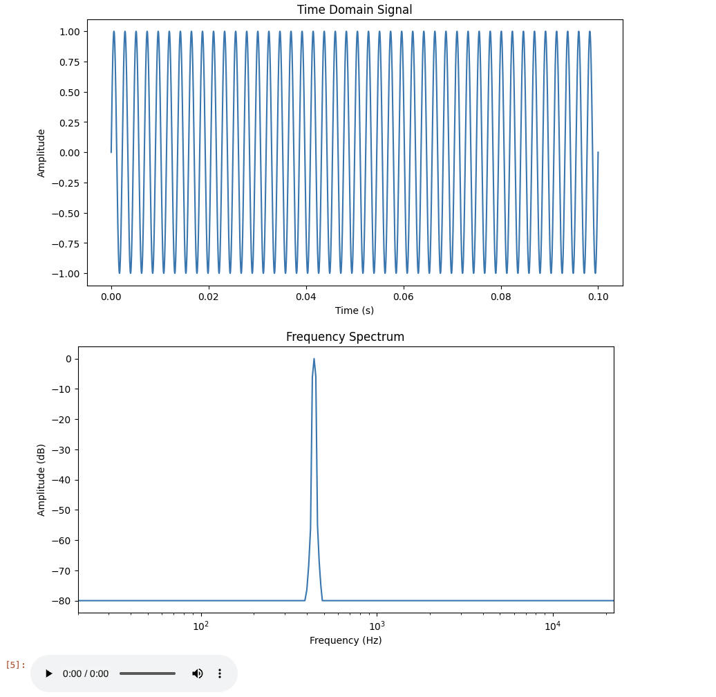
freq = 440 #A4
duration = 0.1
t, y = sine_wave(freq, duration)

time_domain(y, sr)
frequency_spectrum(y, sr)

# playing audio
Audio(y, rate=sr)

freq = 440: measured in cycles per second. 440Hz corresponds to the musical note A4 (often used as reference pitch for tuning instruments).

duration = 0.1: how long the signal lasts. Setting it to 0.1 means the tone will play for 0.1 seconds. Also, if we have $sr=44100$, then the number of $samples = (duration)(sampling rate) = (0.1)(44100)$.

Remember importing from IPython.display import Audio earlier. This is used in Python environments and allows us to directly integrate audio playback features into our notebook.

Output looks like:

By changing the values such as below, we can see how differing the frequency values change the waves and pitch.

t, y = sine_wave(100, 0.1)
display(Audio(y, rate=sr))
[source,python]

t, y = sine_wave(150, 0.1)
display(Audio(y, rate=sr))

# Create a list with three different time durations
durations = [0.1, 0.25, 0.5]

# For loop to iterate through all duration values
for d in durations:
    # Print current duration
    '''YOUR CODE HERE'''
    # Create sine wave with given frequency and the current duration value
    '''YOUR CODE HERE'''
    # Plot sine wave in time domain
    '''YOUR CODE HERE'''
    # Plot frequency spectrum
    '''YOUR CODE HERE'''
    # Play generate sine wave audio
    '''YOUR CODE HERE'''

We do not only have to work with one waves at a time. We can also combine waves:

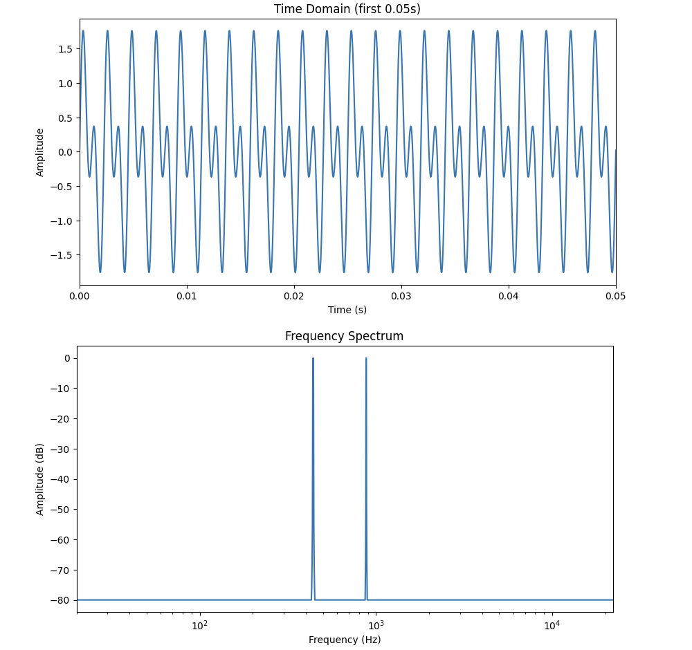
f1 = 440
f2 = 880
duration = 0.5

t, y1 = sine_wave(f1, duration)
t, y2 = sine_wave(f2, duration)
combined = y1+y2

time_domain(combined, sr)

plt.figure(figsize=(10, 5))
plt.plot(t, combined)
plt.xlabel("Time (s)")
plt.ylabel("Amplitude")
plt.title("Time Domain (First 0.05s)")
plt.xlim(0, 0.05)
plt.show()

frequency_spectrum(combined, sr)
display(Audio(combined, rate=sr))

Adding sine waves combines both waves' amplitude and phases, giving us a new waveform. Please try running this yourself, and include the outputs in your project.

You will notice that in this example, the frequency domain plot produces two peaks at 440Hz and 880Hz.

Note that 440Hz (440 cycles per second) sine wave is equivalent to the musical note "A4". This is a fundamental frequency. Then, 880Hz sine wave is called the first harmonic, completing 880 cycles per second (twice as fast as the first one). Musically speaking, this (A5) is an octave higher than A4.

Combined signal can be represented as:

$y(t) = A_{1}sin(2\pi f_{1}t + \phi_{1}) + A_{2}sin(2\pi f_{2}t + \phi_{2})$

$A_1$ is the amplitude of the 440 Hz component ($f_1$), and $A_2$ is the amplitude of the 880 Hz component ($f_2$).

$F\{y_{1} + y_{2}\} = F\{y_{1}\} + F\{y_{2}\}$

Linearity of the Fourier transform implies that each individual frequency component contributes separately to the spectrum. Each sine wave produces a peak at its corresponding frequency in the frequency plot. In terms of magnitude, these contributions add together and do not interfere with one another.

The new shape given by the time domain also makes sense then, because the 440Hz wave has a longer cycle (lower frequency), and 880Hz has a shorter cycle (higher frequency), which is reflected in the faster wiggles you will see inside the bigger overall shape of the time domain graph.

Lastly, for this question, recall from the first signal processing project the RAVDESS dataset. We will explore application of above concept on this dataset.

First load the audio samples as we did in the first project, then pick a sample and output some information about the file like below.

y, sr, filename = load_audio_sample(data_path, "03")

print(f" Loaded: {filename}")
print(f" Duration: {len(y)/sr:.2f} seconds")
print(f" Number of samples: {len(y)}")
print(f" Sample rate: {sr} Hz\n")

Audio(y, rate=sr)

We will break down into sine wave components using Fourier Transform.

num_samples = len(y)
# Compute Fast Fourier Transform of waveform
Y = fft(y) # Time -> Frequency domain

# Get Discrete Fourier Transform sample frequencies
freq = np.fft.fftfreq(num_samples, 1/sr)

# Keep the positive frequencies
freq_positive = freq[:num_samples//2]
mag = np.abs(Y)[:num_samples//2] # How strong each frequency component is
phase = np.angle(Y)[:num_samples//2] # Phase shift in radians

This part lets us analyze the frequency content. You can also write code to visualize the strength of frequencies and phase of each components.

Now try running below code. This is to see what the individual components look like in time domain. Each plot produces top 5 sine waves contributing to the overall audio.

# Pick top 5 strongest frequencies
top_n = 5

# Returns idx of mag sorted in ascending order
indices = np.argsort(mag)[-top_n:] # [-top_n:] gives the last top_n idxs

# Time vector for x axis for plotting sine waves
t = np.arange(num_samples) / sr # np.arange() creates evenly spaced array within specified interval
plt.figure(figsize=(12, 5))

for i, idx in enumerate(indices):
    f = freq_positive[idx] # Frequency of sine
    A = mag[idx] / num_samples # Amplitude
    phi = phase[idx] # Phase

    # Reconsruct sine wave for this frequency compeonet
    sine_wave = A * np.sin(2*np.pi*f*t + phi)

    plt.subplot(top_n, 1, i+1)

    # Plotting first 1000 samples
    plt.plot(t[:1000], sine_wave[:1000])
    plt.title(f"Sine wave {i+1}: {f:.1f} Hz")
    plt.xlabel("Time (s)")
    plt.ylabel("Amplitude")

plt.tight_layout()
plt.show()

You should rewrite the comments in your own words for each part of this code.

Now, we are going to use some sine waves and reconstruct the original sound. This will also show us how much of the audio can be shown through a small portion of frequency components; we can understand what frequencies are dominant in the signal, how frequencies contribute to total waveform, and how increasing the number helps better represent the sound accurately.

# Sort by magnitude
sorted_idx = np.argsort(np.abs(Y))[::-1]

# Number of top frequencies
N_val = [1, 10, 50, 100, 500, 1000]
recons = {}

for n in N_val:
    idx_keep = sorted_idx[:n]
    Y_strongest = np.zeros_like(Y)
    Y_strongest[idx_keep] = Y[idx_keep]
    # Symmetric indices
    Y_strongest[(-idx_keep) % num_samples] = Y[(-idx_keep) % num_samples]
    # Convert back to time domain
    y_rec = np.real(ifft(Y_strongest))
    # Normalize so amplitude belongs in [-1,1]
    y_rec /= np.max(np.abs(y_rec))
    recons[n] = y_rec

# Normalizing
y_norm = y / np.max(np.abs(y))

If the frequency domain data has complex conjugate symmetry, we get real valued time signal back when taking the Inverse FFT (IFFT). So,

$Y[k] = \overline{Y[-k]}$,

where complex conjugates are the frequency bin at index $k$ (positive) and frequency bin at index $-k$.

fft() returns an array with both positive and negative frequencies, where index 0 contains the zero frequency component (DC component), and indices 1 through $N/2$ stores positive frequencies while the latter half stores negative frequencies.

When we only keep Y[idx_keep] part, we are also only taking one side of the symmetry, and to keep the real signal, we need to also set the corresponding negative bins. (-idx_keep) % num_samples is what wraps the negative indices into correct array position. The normalized reconstructions are stored in recons[n]. Let’s plot:

# Move a bit into the audio
start = sr
end = start + 2000

plt.figure(figsize=(10, 6))
for i, n in enumerate(N_val):
    plt.subplot(3, 2, i+1)
    plt.plot(np.arange(2000)/sr, recons[n][start:end], label=f"Top {n}")
    plt.plot(np.arange(2000)/sr, y_norm[start:end], label="Original")
    plt.legend()
plt.tight_layout()
plt.show()

np.arange(2000)/sr creates an array of 2000 elements, and dividing by sr converts into seconds. Each element is a representation of time in seconds corresponding to each sample.

recons[n][start:end] is the reconstructed audio signal. start:end sets the portion we want to visualize.

You should also write the code to output and listen to the audio for each reconstructions.

Deliverables

Although the number of deliverables here seems high, a very large portion of it is simply a repetition of what we did in practice within the problem itself.

2a. Code to plot time-domain, frequency-domain, and play the sound using Audio(). Explain your observations of both Time Domain and Frequency plots. What are some differences?
2b. Provide code and outputs using a different frequency value, and a different duration value. Explain how and why the plots change.
2c. Code and output of (file name, duration, number of samples, and sample rate) loading in an audio sample from the RAVDESS dataset.
2d. Code and output computing FFT, finding strongest frequency components, reconstructing signals, and plotting all examples. You must include comments and explanation of all code, in your own words.
2e. Code and output of the actual audio for all reconstructions using Audio(). Explain how fft() and ifft() are used, and how the resulting audio changes.

Question 3 (2 points)

In this question, we use an example audio file ("brahms") from the librosa library. You can see more about the example files from librosa page. Let us start with plotting:

y, sr = librosa.load(librosa.ex("brahms"))

plt.figure(figsize=(10, 5))
librosa.display.waveshow(y, sr=sr)
plt.title("Time-Domain")
plt.xlabel("Time (s)")
plt.ylabel("Amplitude")
plt.show()

librosa.display.waveshow() is another way to visualize our waveform in the time domain. It takes in an audio time series and the sampling rate (sr) as inputs.

Our previous signal processing project briefly covered spectrograms. Let’s generate a spectrogram for this audio example as well. You can use below functions to help you do this part.

librosa.stft(): computes the Short Time Fourier transform (STFT) of the audio signal. Similarly as before, this applies DFT to each audio frame window.
librosa.amplitude_to_db(): converts amplitude spectrogram to decibel scaled spectrogram.
librosa.display.specshow(): visualizes different audio signal representations.

# Compute STFT of audio time series using librosa
'''YOUR CODE HERE'''
# Convert amplitude to decibels
'''YOUR CODE HERE'''

The next visualization we will explore is a Chromagram. We will generate the chromagram using Constant Q Transform.

chroma = librosa.feature.chroma_cqt(y=y, sr=sr, hop_length=512)

plt.figure(figsize=(10, 3))
librosa.display.specshow(chroma, x_axis="time", y_axis="chroma")
plt.colorbar(label="Intensity")
plt.title("Chromagram (Brahms)")
plt.tight_layout()
plt.show()

A chromagram is a visual representation of the energy distribution of the twelve pitch classes: {C, C#, D, D#, E, F, F#, G, G#, A, A#, B}. Chroma features let us see the harmonic progression of the audio signal.

Deliverables

3a. Load in the librosa audio file of your choice and generate time-domain and frequency spectrum. Include documentation.
3b. Code generating Spectrogram and the audio of the example file.
3c. Code generating Chromagram using CQT.
3d. In your own words, explain what CQT is.

Question 4 (2 points)

Librosa provides various ways to manipulate and analyze audio signals. Some common submodules, and the ones used here include librosa.effects, librosa.feature, and librosa.onset (Read about and discover more functions from librosa tutorial page).

We will take a look at some examples together:

y_time_stretch = librosa.effects.time_stretch(y, rate=1.5)
Audio(y_time_stretch, rate=sr)

Above code modifies the audio signal speed without affecting the pitch. Now, we will try modifying the pitch. Try looking into librosa.effects.pitch_shift() - this is a function in librosa that will help us keep duration the same while modifying the pitch.

# Shift pitch five semitones upwards
'''YOUR CODE HERE'''

Our next example is beat detection. We can perform beat tracking using Librosa as shown below.

tempo, beat_frames = librosa.beat.beat_track(y=y, sr=sr)
beat_times = librosa.frames_to_time(beat_frames, sr=sr)
print(f"Tempo: {tempo} BPM")
print(f"Beat Times: {beat_times}")

librosa.beat.beat_track() returns 'tempo' and 'beat_frames', which are the estimated global tempo (BPM) and the frame indices of beats, respectively. Basically, there are three main steps to how Librosa computes beat tracking. It starts by computing the 'onset strength envelope' using the raw waveform, measuring increases in spectral energy. Then, the tempo is estimated by looking for strength and pattern in onset, then Librosa uses dynamic programming to select beats. Both strength and consistency with the estimated tempo are considered.

We then use librosa.frames_to_time() to convert the frames into seconds. The positions will also be more human readable after this.

# Similar beat detection code but using 1.5 times speed of the original audio
'''YOUR CODE HERE'''

The last example we will see is onset detection. Onset is when the new sound begins.

librosa.onset.onset_detect() finds onset through computing an 'onset strength envelop', where for each time frame it finds out how much energy changes across fequencies. It looks for the peaks, and returns the estimated positions (which intuitively makes sense - we could generally assume that is related to new sound events (biggest sudden increase in energy)).

onset_frames = librosa.onset.onset_detect(y=y, sr=sr, units='time')
# Convert onset frames to time
onset_times = librosa.frames_to_time(onset_frames, sr=sr)
print("onset times:", onset_times)

After you write the above code, you will write code that finds the notes at each of the onset.

onset_times = librosa.onset.onset_detect(y=y, sr=sr, units='time')

# librosa.pyin estimates fundamental frequency
# C2 = second octave, C7 = seventh octave
f0, voiced_flag, voiced_prob = librosa.pyin(y,fmin=librosa.note_to_hz('C2'),
                                            fmax=librosa.note_to_hz('C7'))

# Valid pitch (take nan out)
valid_idx = ~np.isnan(f0)
f0_clean = f0[valid_idx]

# Convert frequency to notes
notes = '''YOUR CODE HERE'''

# Array of time indices corresponding to all the points in f0 array - only on the valid frequencies
times = '''YOUR CODE HERE'''

# Get nearest detected pitch
for onset in onset_times:
    idx = np.argmin(np.abs(times - onset))
    print(f"Onset = {onset:.2f}s | {notes[idx]}")

Below are some explanation of some function we use and/or might be helpful in writing this part of the code.

librosa.pyin() - Function that finds the fundamental frequency in audio signals.

hz_to_note() - Function that finds the nearest note name given one or more frequencies in Hz

times_like() - Function returning array of times in second, matching each frame of feature

Deliverables

4a. Please include the output of the time stretch example.
4b. Code and output for pitch shift example.
4c. Code and output for the beat detection example, using 1.5 times speed of the original audio.
4d. Required code and output for finding notes using onset detection, using hz_to_note() and times_like().

Question 5 (2 points)

Dynamic Time Warping (DTW) finds an optimal alignment between two given sequences. DTW is used in audio and music analysis, and many areas of signal processing, such as beat tracking, melody alignment, sound detection, and speech recognition which is what is was originally created for.

Mathematical Concepts Behind DTW

Given two feature sequences,

$X = (x_{1}, x_{2}, …, x_{n}), \ Y = (y_{1}, y_{2}, …, y_{m})$.

DTW computes the minimum cumulative distance between them. The cost matrix is defined with $C(i,j)$ (size $n$ by $m$) and is calculated using a distance metric, for example Euclidean, or in our case, cosine distance.

$C(i,j) = d(x_{i}, y_{j})$

$D(i,j)$, accumulated cost matrix, is then created, where each element is the minimum cumulative cost. We want to find path minimizing the total cumulative cost while not violating the sequential ordering.

$D(i,j) = C(i,j)
min \begin{cases} D(i-1,j)\\ D(i,j-1)\\ D(i-1,j-1) \end{cases}$

Above cases corresponds to moving down (only X moves/Y is stretched), right (only Y moves/X is stretched), and diagonal (both are advanced (aligned)).

We then find the optimal warping path that minimizes the total cost by backtracking from $D(n,m)$ to $D(1,1)$, picking the lowest cost each time.

$ W = \{(i_{1}, j_{1}), (i_{2}, j_{2}), …, (i_{L}, j_{L})\} $

There are some constraints DTW can not violate:

We start at $(1,1)$ and end at $(n,m)$,
$i$ and $j$ always increases (monotonically increasing),
Each step is one of $(0,1), (1,0), (1,1)$.

We will try DTW on the original example audio and the sped up version.

original_chroma = librosa.feature.chroma_cqt(y=y, sr=sr, hop_length=1024)
fast_chroma = librosa.feature.chroma_cqt(y=y_time_stretch, sr=sr, hop_length=1024)

Below code computes a cost matrix between frames of the two sequences, and returns wp (warping path), aligning frames of the fast version to that of the original version.

D, wp = librosa.sequence.dtw(X=original_chroma, Y=fast_chroma, metric='cosine')
wp_s = librosa.frames_to_time(wp, sr=sr, hop_length=1024)

plt.figure(figsize=(10,5))
librosa.display.specshow(D, x_axis='time', y_axis='time', sr=sr, hop_length=1024)
plt.plot(wp_s[:,1], wp_s[:,0])
plt.title('Question 5 DTW')
plt.xlabel('fast time(s)')
plt.ylabel('original time(s)')
plt.tight_layout()
plt.show()

Let’s walk through above code step by step.

D, wp = librosa.sequence.dtw(X=original_chroma, Y=fast_chroma, metric='cosine')

The function computes DTW and path backtracking on the two feature sequences. D is the accumulated cost matrix computed by DTW, where $D[i,j]$ is the minimum cumulative cost to align first $i$ elements of the original ($X$) with the first $j$ elements of the fast ($Y$). wp is the warping path, which is an array of $(i,j)$ pairs corresponding to the minimum cost alignment start to finish.
metric='cosine': calculates distance between feature vectors, which is used to create the DTW cost matrix.

$distance(a,b) = 1 - \frac{a \cdot b}{||a||||b||}$.

Setting this matrix gets the cosine distance for each $C(i,j)$ after DTW function establishes the cost matrix $C$; we get the distance between the $ith$ feature vector of the first sequence and $jth$ feature vector of the second sequence. The accumulated cost matrix $D$ uses the cosine distance for each $D(i,j)$ to get the cost to that cell from $(0,0)$.

If you have heard of cosine similarity (or as we used in some of our previous projects), you might notice that this formula looks similar to that of cosine similarity. It is indeed derived from cosine similarity, but changed so that we are computing distance instead of orientation of vectors. Cosine similarity ranges from -1 to 1, where -1 means they are opposite (most dissimilar). In cosine distance,

0: vectors are identical in direction

$cos(\theta) = 1 \rightarrow d = 0$

1: vectors are perpendicular

$cos(\theta) = 0 \rightarrow d = 1$

2: vectors are opposite

$ cos(\theta) = -1 \rightarrow d = 2 $

wp_s = librosa.frames_to_time(wp, sr=sr, hop_length=1024)

This converts wp into the corresponding time in seconds, given the sampling rate and hop length.
Thus, note that with wp being the path returned by librosa.sequence.dtw, we would have $wp = [[i_0 ,j_0]. [i_1, j_1], …]$. $i$ is the frame index in $X$ and $j$ is the frame index in $Y$. Then, each row tells us where a $X$ frame aligns with $Y$. It also follows that $wp_s$, after getting the time in seconds, gives us a 2D array $wp_2 = [[t_i0 ,t_j0]. [t_i1, t_j1], …]$.

Time is calculated using below formula:

$time = frame \ index \cdot \frac{hop \ length}{sampling \ rate}$

hop_length: specifies the sample offset between consecutive frames. This is also the difference between a frame’s start time and the next frame’s start time.

frames_to_time should use the same hop length for accuracy.

librosa.display.specshow(D, x_axis='time', y_axis='time', sr=sr, hop_length=1024)

This line displays the DTW accumulated cost matrix $D$. We label the axes in seconds, and sr=sr sets the sampling rate of audio (used in frames to time conversion), and 'hop_length=1024' specifies the step of the frame.

ax.plot(wp_s[:, 1], wp_s[:, 0])

This puts the warping path on top of the cost matrix image.

plt.plot(wp_s[:,1], wp_s[:,0])

This line plots the optimal path on top of the cost matrix. wp_s[:,1] is the $x$ coordinates and wp_s[:,0](fast audio time) is the $y$ coordinates (original audio time).
The output will be a plot showing alignment relationship between two sequences. If the line deviates from the diagonal, one of the sequence is stretched/compressed relative from the other.

Once you run the code, you should see the output that looks like the plot below:

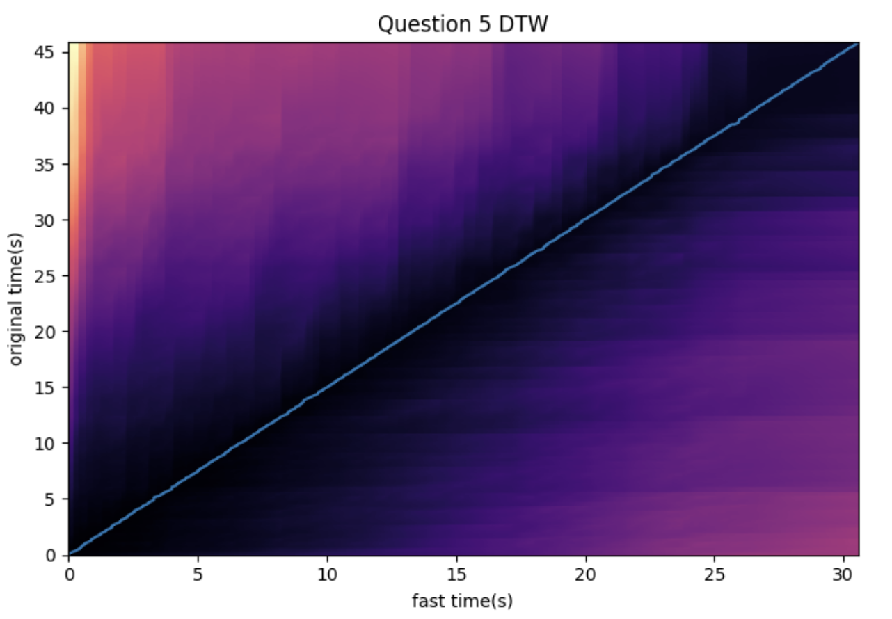
Remember that we used the two chroma sequences taken from the original audio and the fast audio which was a time stretch by $1.5x$. Then, the near linear line we see in the graph makes sense, because with x = fast time and y = original time, the slope a greater than 1 suggests that the original time is approximately the fast time multiplied by a constant.

The darker areas represent lower cumulative costs (better alignment), while lighter areas represent higher cumulative costs (worse alignment).

Deliverables

5a. Explain in your own words what DTW does and briefly explain how it works.
5b. All running code and output of DTW example.
5c. Why does the first example result in a near linear looking line and what does that imply? Write a few more sentences about your other observations and interpretation of the output.

Question 6 (2 points)

Continuing from our DTW example, we apply the same method to our dataset audio. First, modify the load_audio_sample slightly so we can collect all the happy emotion audio files.

def load_audio_sample(data_path, emotion_code):
    #
    samples = []
    for root, dirs, files in os.walk(data_path):
        for filename in files:
            if filename.endswith('.wav'):
                parts = filename.split('-')
                if parts[2] == emotion_code:
                    file_path = os.path.join(root, filename)
                    y, sr = librosa.load(file_path, sr=None)
                    samples.append((y, sr, filename, file_path))
    return samples

happy_samples = load_audio_sample(data_path, emotion_code="03")
for y, sr, fn, fpath in happy_samples:
    print("Loaded:", fn, "sr:", sr, "len:", len(y))

Then, we pick the two audio frames we will be comparing (Feel free to pick two samples of your choice from the happy audio files; however, try to pick two audio samples that sound noticeably different).

# First audio sample
y1, sr1, fname1, fpath1 = happy_samples[0]

# Second audio to be compared with first
'''YOUR CODE HERE'''

# Code to listen to both samples
'''YOUR CODE HERE'''

Similar to what we did in question 5, we will compute the chromagram features for each audio.

hop_length = 1024
# Using y1
chroma1 = '''YOUR CODE HERE'''

# Using y2
chroma2 = '''YOUR CODE HERE'''

# Get the accumulated cost matrix and optimal warping path using librosa.sequence.dtw().
D, wp = '''YOUR CODE HERE'''

# Convert frame indices to time in seconds using
wp_s = '''YOUR CODE HERE'''

# Code to plot accumulated cost matrix and optimal warping path
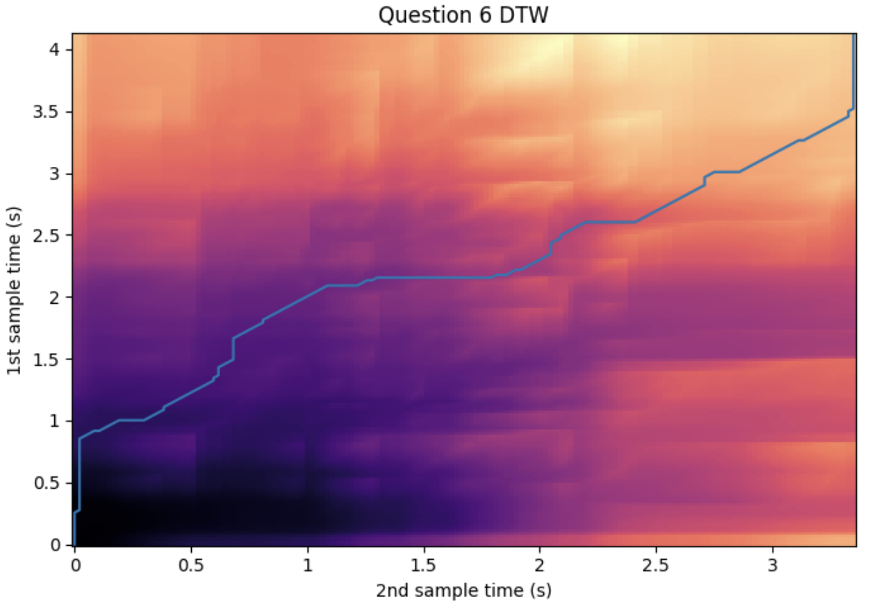
'''YOUR CODE HERE'''

For example, choosing samples at index 0 and 22, we can see the output as such:

Deliverables

6a. Modification of the load_audio_sample function. Make sure to write comments.
6b. Code and output of audio and audio information of the two examples chosen.
6c. Completed code for computing chroma features and DTW.
6d. Code for plotting. Make sure you have the output included.
6e. Write a few sentences regarding your observation and interpretation of the output.

Submitting your Work

Once you have completed the questions, save your Jupyter notebook. You can then download the notebook and submit it to Gradescope.

Items to submit

firstname_lastname_project7.ipynb

It is necessary to document your work, with comments about each solution. All of your work needs to be your own work, with citations to any source that you used. Please make sure that your work is your own work, and that any outside sources (people, internet pages, generative AI, etc.) are cited properly in the project template.

You must double check your .ipynb after submitting it in gradescope. A very common mistake is to assume that your .ipynb file has been rendered properly and contains your code, markdown, and code output even though it may not.

Please take the time to double check your work. See here for instructions on how to double check this.

You will not receive full credit if your .ipynb file does not contain all of the information you expect it to, or if it does not render properly in Gradescope. Please ask a TA if you need help with this.