TDM 20200: Project 7 - Introduction to Steganography & Steganalysis

Steganography is the art and science of hiding information within otherwise non-secret data. You can accomplish this by subtly modifying pixel values. The Least Significant Bit (LSB) method is one of the simplest and most intuitive approaches.

Key Concept: Each pixel in a grayscale image has a value from 0-255 (8 bits). The least significant bit (rightmost bit) contributes the least to the visual appearance. Changing it from 0 to 1 (or vice versa) changes the pixel value by at most 1, which is imperceptible to the human eye.

For example:

This is a subtle change, but it is enough to hide a message while staying hidden.

Since images are just composed of a bunch of pixels, which are in turn composed of bits, we first need to convert our message to binary before we can hide it in the image. Each character of our message can be decomposed into 8 bits. We will also need a special "delimiter" to mark where the message ends in the image so we do not accidentally decode a message that is not intended for us.

Let’s start by converting our message to binary and adding our delimiter:

Let’s now take a quick look at what our message actually looks like in binary:

Looks like binary to us! Also note the delimiter we added to the end of our message.

But what if our message is too long? We would not be able to fit it into the image since our upper bound of how long a message can be is the dimensions of the image. So, let’s load up an image and check to make sure it can fit with our approach:

Looks good! This means we should be able to fit our message into the image which we can quickly visualize like so:

Also note that unlike our message, our image is a 2D array composed of pixels. So we will need to flatten our image to a 1D array of pixels so we can modify the LSBs of each pixel sequentially.

Now that, we have our message in binary, we need to modify the LSBs of each pixel in our image to hide our message. To encode a bit into a pixel’s LSB, we need to:

There is a pretty cool trick we can use to modify the LSB of a pixel. If we take the pixel value and then AND it with 0xFE (which is 11111110 in binary), we clear the LSB. Then we can OR it with our message bit to set the LSB to the desired value: (pixel_value & 0xFE) | message_bit.

We will use this logic in the next section to implement the full encoding function.

Our last step is to implement the full encoding function using similar logic to what we did above. Most of the code is provided - you just need to fill in the critical part where we modify the LSBs.

Please test your function with the following message:

Please print the original and stego-image arrays side-by-side for the first 10 pixels to ensure the LSBs were modified correctly.

You can also check that only the LSBs changed by using the bitwise XOR operator ^ to compare the original and stego-image arrays and then applying the bitwise AND operator & with 1 to get the LSBs. For example, the second pixel in the original image is 204, but it becomes 205 in the stego-image which this line of code verifies:

Now that we can encode messages into images, we need to decode them! Decoding is simpler: we just extract the LSBs from each pixel and convert them back to characters.

To decode, we can peform the encoding logic in reverse:

To extract the LSB from a pixel, we can use a simple bitwise operation: pixel & 1 which will give us the rightmost bit of the pixel.

Please fill out the function below to decode the message from the stego-image:

Once you filled out the function, please test it out with the image we encoded our short_message into last question to see if you get back the correct result!

So far we haven’t actually seen what the stego-image looks like. So now let’s compare the original and stego-image visually but also quantitatively! We can visualize this by plotting the images side-by-side.

But first, let’s also use a slightly more complicated message to encode and decode since our previous message was too short to really see the difference:

Please use this message with your encode and decode functions and show the decoded message output. Note that since this message is so long we will need to truncate it when using the basic LSB approach (try the first 20,000 characters).

Let’s now plot the original, the short stego-image, and the long stego-image side-by-side to see if we can visually detect any difference:

We should not see much if any difference between the original and stego-image but that is exactly what we want! We can also use some simple metrics to quantify the difference between the two images which may help us understand how well our steganography technique is working.

MSE (Mean Squared Error) and PSNR (Peak Signal-to-Noise Ratio) are common metrics used to evaluate the quality of steganographic images. MSE quantifies the average error between corresponding pixels, while PSNR gives a sense of the overall visual quality—higher PSNR means the images appear more alike. PSNR expresses the ratio of the maximum possible pixel value to the square root of the MSE which allows us to get a sense of the perceptual quality of the images since it uses the same units (pixel values).

Let’s implement it in code and see what we get:

We should see a very small MSE (typically 0.0001 to 0.01 depending on message length) and a higher PSNR (typically 40-60 dB). This means the images are nearly visually identical to the original natural images, which is exactly what we want and is the basic goal of steganography! The small MSE reflects that we only changed the LSBs of some pixels (each change is at most 1 in pixel value), so the average squared difference is very small.

Notice that even though we cannot visually detect a difference between the original and stego-image, the PSNR is lower for the long stego-image which is expected since we are encoding way more information into the image. However, more complex methods should allow us to encode more information into the image while still maintaining a lower MSE and higher PSNR.

So far we have used only 1 bit per pixel to keep our changes as subtle as possible. But consider that even though we can use more bits in every pixel to store more data, the more bits we modify the larger the changes visually. A very similar approach to the one we just used is to use the last n bits of each pixel to store our message. This is known as n-LSB encoding and is a very simple and effective way to encode more information into the image while still maintaining a relatively high PSNR.

However, it is not a very elegant solution and is still relatively easy to detect which we can see in the following images:

Now using 5-LSB might be exaggerating here, but you can see that the visual difference is much more noticeable - there are actual major areas that are noticeably "off". But, even with smaller values of n, this method can still be very easily detected using statistical methods.

Another way to approach encoding more information in an image is using some form of dynamic analysis to decide where you can reasonably encode more information. This stems from the fact that some images are "messier" by nature - think of a picture of Times Square at night versus a picture of a simple grass field and with a clear blue sky. The picture of Times Square has more going on all the different lights, advertisements, people, cars, etc. compared to the simplistic block of green and block of blue.

In our image, areas like the fauna or some parts of the dinosaurs scales and shadows may have higher variance indicating they might be a better place to encode our message.

With this in mind, we can look at implementing adaptive encoding based on the pixels regional variance to ensure we only modify pixels in a higher variance (or already otherwise noisy) area.

Key Concept: Calculate local variance for each pixel. High variance = textured area (good for hiding). Low variance = smooth area (bad for hiding).

The way we are going to approach this is to first create a variance map in a function called calculate_local_variance(image, window_size=3). We need to create a sliding window or a kernel that can give us the average pixel value in the area surrounding the pixel. This can be done using convolution which is a common operation in image processing.

Take a look at the following gif to see what convolution is and how it works. Different kernels have different effects on the input, for example the one in the gif is a sharpening kernel which makes the image edges more pronounced.

The kernel we are using is a box kernel which is a simple average of the pixels in the area surrounding the pixel (commonly used for blurring images):

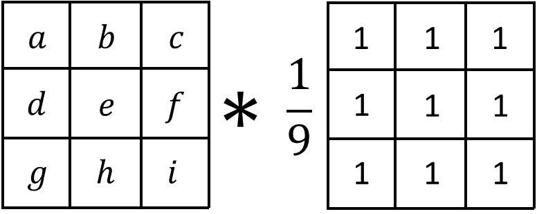
Now we can just calculate the variance (mean square diff of original image as a float and the local_mean). The final step is to convolve this map of squared differences again using the same kernel which gets us the regional variance for that pixel.

Please put these all together into a function that returns the variance_map and then let’s graph the variance map to see where those higher variance areas are:

The outlines of the dinosaurs and faunas are the brightest areas in the variance map indicating they are the areas with the highest variance which means we can reasonably encode more of our message in these areas.

First we want ensure that we can actually fit our message into the image like we have in the past. To accomplish this we can directly compare our variance map to a threshold (map >= threshold) which gives us a boolean map. We can then sum this to get the number of 'suitable' pixels we can modify.

We can then use this to see how many characters we can fit into the image:

Not only that but we can also visualize the suitable pixels to see where we can encode our message:

It looks like there are quite a few suitable pixels to encode our message in which means we should be able to fit a longer message into the image!

We can then use a pretty slick numpy function called np.where() to get a list of all the indices that we classified as suitable:

We can now iterate over and then modify the bit like we did before:

Using the above, please fill out the rest of the implementation:

Note this adaptive LSB implementation is currently only handling 1-LSB but you can definitely modify the logic to have more complex thresholds allowing you to encode 1, 2, or 3-LSB (or more) into your image giving it a much higher capacity.

Now please also calculate the PSNR of the adaptive encoded image as well and compare to the basic LSB encoding.

We can also visualize the before and after side by side to see the difference:

So far we have talked about different ways to encode messages into images, how to decode them and mentioned how certain methods are more discrete than others. But how can we actually detect if a message has been hidden in an image? This is where steganalysis comes in!

Steganalysis is the detection of hidden messages. Even though the goals of the methods we have discussed so far is to remain visually imperceptible, LSB in particular, leaves statistical traces that can be detected!

When we perform LSB steganography, we’re modifying the least significant bit of pixel values. This creates a specific statistical pattern that can be detected through histogram analysis which can be referred to as the pairing effect.

But why do these pairs form?

Consider what happens when we modify the LSB of a pixel:

The key insight is that when we randomly modify LSBs to encode a message:

However, in a natural image, there’s no real reason why 150 and 151 should have similar counts which is why we can use a histogram approach to reveal this pattern!

What to look for:

When plotting histograms, you might notice that pairs of values appear more balanced in stego-images compared to originals, especially in regions where many pixels were modified. This can indicate that someone tampered with the image to hide some information in it!

Looking at a more concrete theoretical example:

Imagine an original image has these pixel value counts:

After encoding a random message using LSB steganography (modifying ~50% of pixels with values 150 or 151):

The histogram would show the pair becoming more balanced, which is suspicious for a natural image!

So now let’s analyze histograms on our images to detect these patterns by calculating the histogram and basic statistics of the image.

Go ahead and call the analyze_histogram() function on the original and stego-image and print the statistics. But curiously enough, when you just look at the statistics, it looks like the stego-image is actually very similar to the original image!

Let’s go ahead and use the histograms we just got here to compare the histograms of the original and stego-image:

Now here is where we see the difference between the original and stego-image histograms. Notice how the original histogram shape looks much smoother and more natural compared to the stego-image histogram which seems to have a bunch of spikes all throughout the histogram. If we were to plot an image and see patterns like this, it would be a strong indicator that something is hidden in the image!

Histogram analysis is not foolproof and has a few important limitations:

But even with limitations, histogram analysis is still a useful tool to detect hidden messages in images and it also motivates the development of more sophisticated steganographic methods (like adaptive encoding and DCT-based methods) that are harder to detect.

We have previously only worked in the spatial domain (directly modifying pixel values) which we saw in the last question can be detected relatively easily with histogram analysis or other simple statistical methods. Now we will explore something a little more interesting: the frequency domain!

In this approach we look to decompose the image into its frequency components, hide information in the transform coefficients, then transform it back to the spatial domain ideally achieving a more naturally distributed message across the image making it more difficult to detect.

Why frequency domain?
- More robust to compression (like JPEG)
- Can hide in less perceptually important frequencies
- Harder to detect with simple statistical methods like the histogram-based analysis from the previous question

We will explore a common frequency domain transformation: the Discrete Cosine Transform (DCT) as means of hiding information in the frequency domain.

What is DCT? DCT converts an image from spatial to frequency representation. It’s the same transform used in JPEG compression!

Key Concept:
- Low frequencies = smooth changes, things like brightness, contrast, and other low-frequency changes that are important for visual quality
- High frequencies = sharp edges/details, less important, often lost when compressing images like JPEG
- Mid frequencies = good place to hide data (not too important, not too noisy), this is where we will modify the coefficients to hide our message

DCT works on 8*8 blocks:

Looking at this example, we can see the general idea of how the image is broken up into blocks and then each block is transformed into its frequency domain representation like shown in the image on the right.

This is a closer look at a single block transformed into its frequency domain representation:

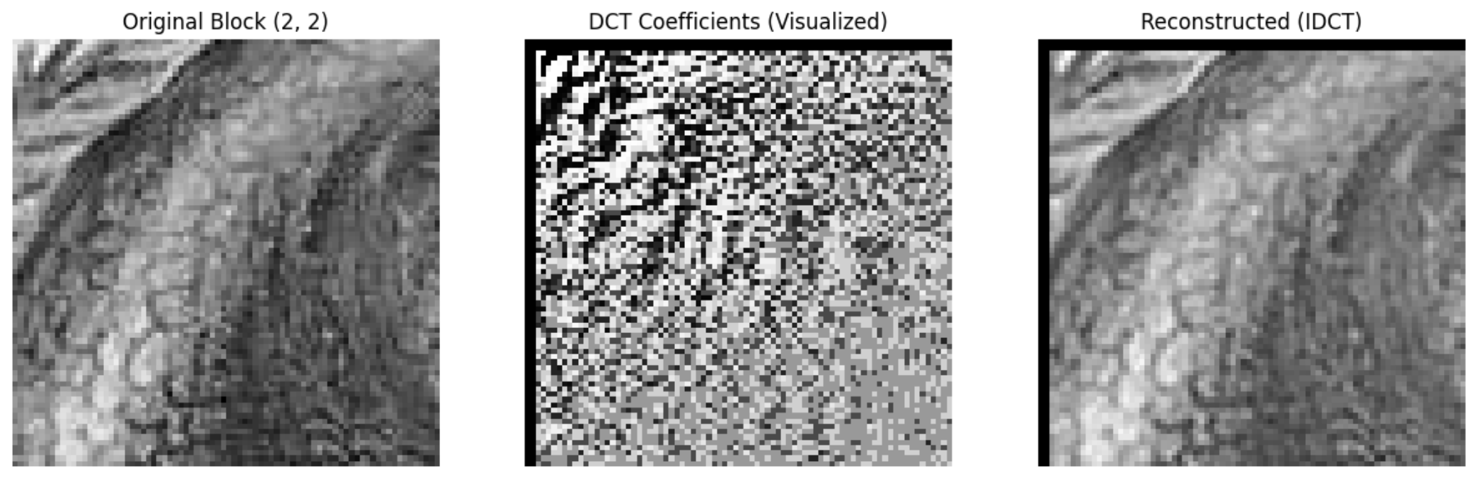
We then modify these coefficients to hide our message and then transform it back to the spatial domain to get the stego-image. In this example, there is a noticeable difference between the original and stego-image. But, note that this is showing the DCT blocks on a much larger scale than what we would be doing in practice, and, as a result, the differences are more noticeable.

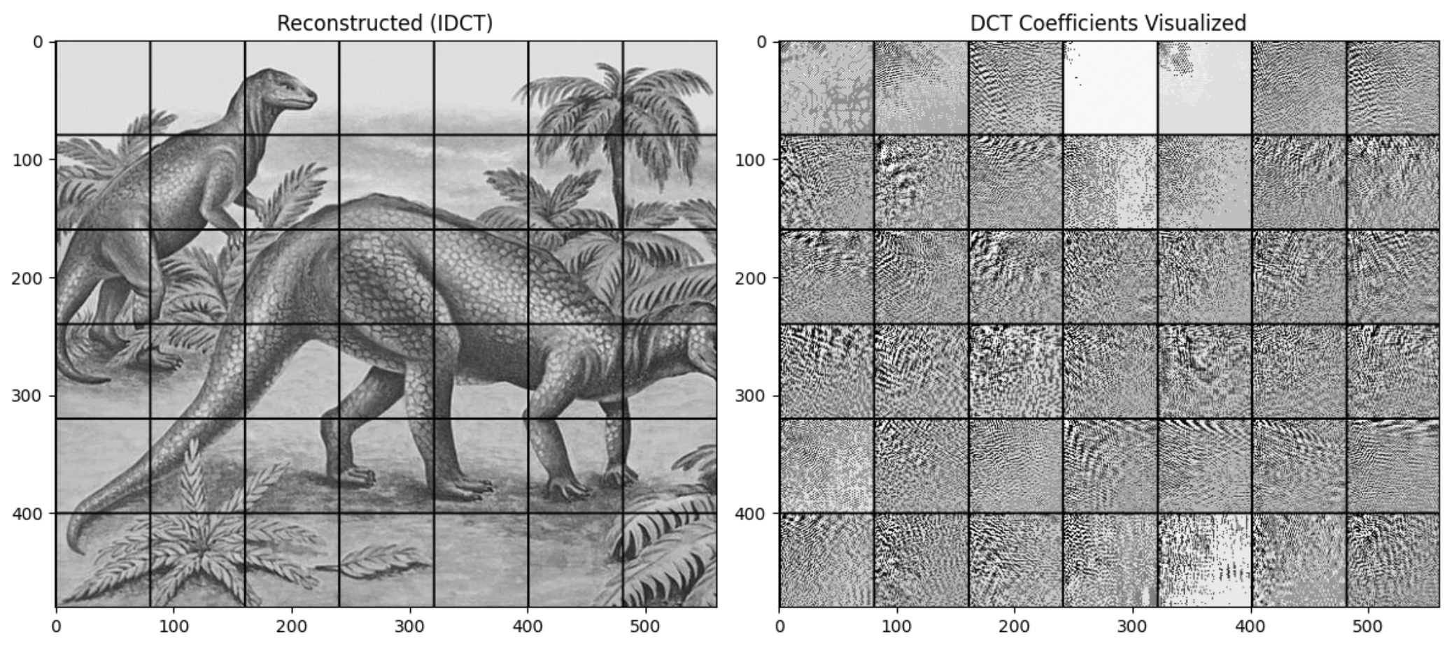
In reality, the image would be broken up into many more blocks (8x8 pixel chunks) as opposed to the entire image in an 8x8 grid to look something more like this:

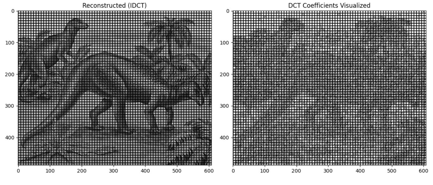
Here you can, just by looking at the representation of the coefficients, still see the general shape of the image. Splitting the image this granularly gives us more fine grained control over the image.

The code to produce these graphswas adapted from this link and converted into Python3 to visualize the DCT coefficients of the image.

Now let’s actually go to encode a message into the image using the DCT coefficients.

The implementation below has most of the tedious parts filled out like converting the message to binary and padding the image to be multiples of the block size, etc. but we are going to focus on the part where we modify the coefficient due to numerical precision issues when doing these transformations on such a large scale.

One thing to note is that in DCT steganography, we don’t use the same concept of delimiters for a few reasons primarily dealing with numerical precision issues when doing these transformations. Instead we state at the beginning of the message how long the message is in bits and then we encode the message bit by bit.

Like we mentioned earlier, the mid-frequency coefficients are the good place to hide our message so we are going to isolate one of the the mid-frequency coefficients (position 3,4) and check if it is able to store our message based on if the absolute value of the coefficient is larger than some threshold (e.g., 1 or 1.5 - this is based on the ranges of the coefficients).

If yes, we first want to preserve the sign of the coefficient and then modify the coefficient to encode the bit: round the coefficient and set LSB like we did in the previous questions. If no, skip this block.

We can now test the encoding function with a message, but we should note that the current implementation has a very low capacity since we are only modifying one coefficient per block meaning we really only have capacity for around 4-5k bits in this image. There are ways to improve this by modifying more coefficients per block using more advanced techniques like the zigzag scan which you can read more about in this discussions post.

Decoding DCT is actually even simpler for a couple reasons: the first block tells us exactly how long the message is meaning we do not need to worry about delimiters and we do not need to worry about redoing the transformations to get the original image.

Similar to the LSB decoding function, it is simply the reverse logic of the encoding function:

Now let’s test the decoding function with the stego-image we encoded our message into:

You should see that the decoded message matches the original message!

The nice thing about DCT is that is a very common and powerful transform that is used many other places other than steganography like in image processing and image compression (JPEG). Hopefully this project provided a useful introduction to some of these concepts!