TDM 40200 Project 9 - Cross Validation

Before getting started, let’s understand what we are working with and what we need to prepare. We have done a lot of data exploration and cleaning throughout the Data Mine projects; we will follow a similar process here.

Please start by printing the head, shape, and columns of this dataset.

You will also almost immediately notice only from the head that there seem to be quite a few missing values. Let’s take a deeper look into that by counting the number of NaN in each column:

The output will indicate that the dataset has many missing data, which is not abnormal for a health and survey dataset especially where not all participants will complete every single exam, but we should handle it appropriately.

We will not just simply drop all rows with missing values using df.dropna() as we will lose most of the data. Instead, we will select a subset of relevant predictors, with our target being heart attack. Please use the following features.

The columns representing diseases, are coded in the NHANES dataset, seen at the table below:

We can check that ourselves too.

Above is an example output for Heart_attack only, and you will notice similar output with same coded values for other conditions as well. This confirms the NHANES coding scheme.

For us, values 7 and 9 are invalid so they will be removed.

Now we recode into a binary variable, such that 1 is for heart attack, and 0 is for no heart attack.

Now we will select the variables and drop missing values only for the used variables in this project.

This question will give a motivation into Cross Validaiton.

Now that we have the cleaned data, we will build a model using KNN. KNN is a simple algorithm that classifies points using the k-nearest training examples and a majority vote. The number of neighbors is defined with 'k'.

First, split features and target in the data by:

KNN will calculate the distance between points and is sensitive to distance and scaling; without scaling, large scale variables will deominate calculations. StandardScaler shifts the data so the mean is 0 and standard deviation is 1, ensuring all features contribute equally. To do so, we need to import:

For Train/Test split, import the following package:

Split the data into 80% train and 20% test using train_test_split after scaling features:

Now we are ready to train the KNN model. Scikit-learn library provides the KNN algorithm class. The second import will be used later to calculate the accuracy of classification models.

Now we want to measure how well the model worked.

With a very broad explanation, overfitting happens when a model learns the training data too closely and performs poorly on new data, while underfitting occurs when the model is too simple to capture the underlying pattern in the data. The following code chunk trains a KNN model for different values of k, computes accuracy on both training and test data, and stores the results to compare model performance.

To get a better idea of what insight this provides us with, we can visualize this result as well. Please also write code to plot both training and test accuracy scores against k values in the same figure. You should see a plot like below as the output:

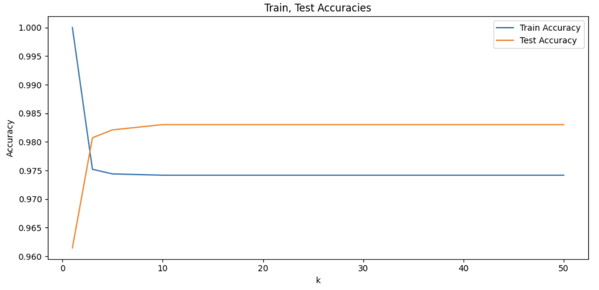
At the beginning of the graph, train accuracy is at 1.0, while being the same point where the test accuracy is the lowest. As k increases, train accuracy starts decreasing while testing accuracy starts increasing. With more neighbors, the model averages out data and noise better by being aware of broader patterns. Test accuracy seems to peak around k=10. As k continues to increase, we can notice the plateau; increase in number of neighbors is no longer effective in improving model’s accuracy and k values have become too large that it captures much of the global structure.

In other words, very small k values cause overfitting and large k values cause underfitting. Overfitting is when the model is very sensitive to local details and noise, and underfitting is when the model is too general and fails to capture specific patterns of the data.

The problem arises when, by chance, we obtain an unbalanced or unrepresentative train/test split. Depending on which rows we randomly land in validation set the accuracy can vary. A particularly easy or hard validation set would lead to error that does not accurately reflect true data.

We can illustrate this by training the same model multiple times on the same dataset.

The output is:

The accuracy scores range differently although the model and data are the same. This single split approach gives us one outcome from a distribution of possible scores and we would not know which. Other important considerations is that we are also losing parts of data that could have been taken into consideration during training as 20% of the data is set aside, and we could end up with validation error that does not accurately reflect true data as an unlucky split can lead to a wrong selection.

This is where Cross Validation comes in.

K-Fold Cross Validation divides the data into K equal-sized folds. In each round, training is done on K-1 folds and the remaining fold is used for validation. The K validation scores are averaged to get a single estimate of the model’s performance.

We will continue to use Scikit-Learn. Scikit-Learn handles the entire cross validation process through cross_val_score function (see cross_val_score documentation for more details).

KFold class creates the indices to split the data into train and test sets. It splits the dataset into k partitions.

`KFold`class creates the indices to split the data into train and test sets. It splits the dataset into k partitions (see KFold documentation for more details).

Below, we create KNN classifier and define our cross validation strategy. The dataset is split into 10 equal sized folds.

We also manually set 'shuffle=True' as KFold does not shuffle by default. This allows us to randomize row ordering. If there is no shuffling, the assignment of rows to folds would depend on their original positions; this can be problematic for sorted or grouped datasets, for example by age or dates, as it would lead to unrepresentative folds.

KFold from before just splits the indices. Training and evaluation of the model can not be done without knowing how to split, so we pass in the cv=kf argument.

Note that separating these components also provides flexibility, since cross_val_score() can accept other types of splitting strategy. For example, we can pass in StratifiedKFold or LeaveOneOut() (these will be presented in upcoming questions) instead of KFold.

Here, the model is trained 10 times and accuracy is evaluated for each fold. The function returns an array of scores corresponding to each cross-validation run.

K-Fold is standard, but there are other types of cross validation methods. Leave One Out Cross Validation (LOOCV) is a form of cross validation, where the number of folds is set equal to the total number of samples, n. Only one sample is used for validation per iteration and the remaining n-1 rows are used for training. This repeats until all rows have been used as the validation set once.

Just as an example, suppose we had a dataset with 5 observations. Then,

LeaveOneOut from Scikit-Learn provides the indices for splitting data into training and testing sets.

LeaveOneOut from Scikit-Learn provides the indices for splitting data into training and testing sets (see LeaveOneOut documentation for more details).

Because the training set (size n-1) is almost the entire dataset (size n), we are generally able to obtain a low bias estimate with this method; the model is exposed to nearly all the data in each round. However, this also leads to LOOCV having high variance with the validation set being just a single point, thus very sensitive to outliers and noise.

At this point you might also realize LOOCV can have a high computational cost and is especially inefficient for large data, since the model needs to be trained once for every observation in the dataset.

You should see:

This implies fitting the model 10892 times is required if we are to use LOOCV.

Now, we will apply LOOCV (As previously mentioned, running this may take a couple minutes). Please complete the code below.

Note that we do not need to shuffle here since the concept of folds used in previous cases do not apply here; every single row gets used as test regardless of ordering. We do not see the problem of similar rows grouping into the same fold here.

Additionally, notice that we are just printing the mean and standard deviation of the accuracy. Comparing to regular K-Fold method, we were able to compute meaningful proportion using (Correct Predictions) / (Total in Fold); however, in LOOCV since each validation fold contains one row only, the model predicts either correct or incorrect. If we print the accuracy values, we will obtain an array of only 0s and 1s. You can see it for yourself too (try printing the accuracy value, and you will get: array([1., 1., 1., …​, 1., 1., 1.]) ).

Mean value matters since it is (total correct predictions) / (total number of rows).

Another version of cross validation is Stratified K-Fold Cross validation. You may recall our dataset is imbalanced, with only a small subset of individuals being a heart attack patient. Creating folds randomly may lead to some folds containing very few heart attack cases, resulting in unreliable evaluation results. Stratified K-Fold Cross validation is a way to resolve this type of issue by ensuring same class distribution as the overall dataset, making it particularly useful for classification problems (especially with uneven distributed labels).

StratifiedKFold from Scikit-Learn provides train/test indices for splitting data and keeps approximately the same percentage of target class samples as the original dataset.

You will see output like:

Each number in the score corresponds to the accuracy obtained in one fold. There are 10 since we used 10 folds.

Now, we will compare the class distribution inside each fold to verify that this method actually preserves it. For example, take regular K-Fold and our current Stratified K-Fold.

Output:

Please complete code below to see such for Stratified K-Fold as well.

Output:

Compare the outputs. In standard K-Fold, the heart attack cases range from 37 to 72 across folds. Model validated on Fold 1 has a set where heart attack patients are very underrepresented, thus the validation score would be unrealiable to be used as a good estimate. But Fold 5 had almost the double. Neither are accurate reflections.

However for stratified K-Fold, we can see that the number of heart attack cases is almost identical across folds. Each fold has about the same number of positive/negative cases.