TDM 40100: Project 11 - Decision Tree

It is expected that the e-commerce market is to reach approximately $8 trillion by 2027, and around 20% of global retail sales are being done online. It is no doubt that online shopping and the e-commerce market continues to grow and is one of the irreplaceable methods in sales. So, it is crucial businesses understand customer behaviours when it comes to online shopping activities and their online experience. This means we need to be able to recognize patterns from the data we have, and find out what factors contribute most to customers deciding to make purchases.

The dataset we will be using contains numerous information about customers and their behaviours in online shopping. It includes features from customer types and dates to demographic and different online activities on the website. Using these data, our goal is to predict revenue and how different features are related to purchases, while understanding how the performance of our model can change and how we can get the best prediction. As mentioned earlier, we will do so by exploring decision tree modelling.

To begin, we will load and print the head of the data. As we always do, we will inspect our dataset before starting any analysis or modelling. First check the head and shape of the dataset. Then, checking for any missing or duplicate values, you should notice that below variables have missing values:

And below variables have duplicates

We will remove missing values and duplicates as a part of this question. We will also convert our categorical variable into indicator variables through one hot encoding. First, check the original data types for each variable.

Now, we will use Pandas library’s pd.get_dummies to perform this task. By doing so, we obtain multiple new columns that take on values either 0 (not present) or 1 (present), and each column represents a unique category. Then, we can represent numerical data using binary conditions, which the tree uses as criteria for splitting.

In this question, we will split the dataset into training and testing. This step is crucial for the decision tree to make good evaluations and not overfit. We can see how well model performs generally, by testing the trained part on new, unseen subset of data that was not used yet. Scikit-Learn has a model_selection module that contains various methods we can choose for evaluating models and tuning parameters. To divide the dataset, we will be using train_test_split.

Let’s split as shown below:

You can think of X_test as the input and y_test as the output. Revenue is what we want to predict, so it is not included in the input features. The test_size is set to 0.2, meaning we are using 80% for training and 20% for testing. random_state controls the seed for random generator. Setting this number also makes sure that the split is reproducible means the same portion of the dataset will be included every time.

Above will train the created decision tree using the previous training data.

Let’s see the predicted outcome for our X_test feature.

Now, as we do with other models, we will explore some methods we can use to determine how well this model performs. Below are the imports needed for this task:

We can evaluate the performance using accuracy score, classification report, and confusion matrix. The code for this looks like:

We got the following output from the classification model:

Accuracy score measures the proportion of correctly classified instances out of the total number of instances in the dataset.

Some main information we can get from the classification report are precision, recall, and f1 score as shown above.

Now for the confusion matrix, from the first row, left to right, it holds the value for true negative, false positive, false negative, and true positive. For our data, respectively, this means:

Let’s take a look at another representation of the confusion matrix. Import the below:

We can use the below code to make the visualization.

The matrix should look like below:

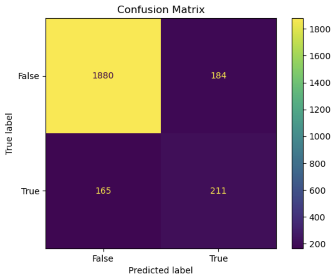
On the x-axis, we display all data points that the model predicted to belong to the selected class (either true or false). On the y-axis, we list all examples with the actual label for that class, for example, row 0 represents customers who actually made “no purchase.”

So again, applying the implication of the different sections of the matrix mentioned previously, we can see that there are 1880 correctly identified non purchase, 184 customers identified to have made a purchase when they did not, 165 missed actual purchases, and 211 correctly predicted purchases.

confusion_matrix() outputs an ndarray of the values, but with ConfusionMatrixDisplay(), we get the plotting object that can be used to visualize it better.

There are various parameters we can adjust to best work with the problem and dataset. We will take a look at max_depth, min_samples_leaf, and criterion.

We will test using the following ranges of parameter values:

We can plot how the values for max depth affect the accuracy of the model.

As with other types of data analysis, we can also visualize the decision tree produced. To do so, make the following import:

Plot the tree using:

There are parameters you can adjust for the tree output. For example, adjusting max_depth will output only the number of depth you want to show in your tree, and other specific namings or preferred visualization.

Additionally, feature importance is a score corresponding to how much each feature contributes to the tree making the decision. The higher the value, the more important the feature is. It is easy to get this value using feature_importances_.

Now, we will make a comparison between users who made a purchase and did not make a purchase. The division is made by the variable "Revenue": if a purchase was made then the value is True, and False otherwise. Common, but useful information we can have is how their behaviour, or the same variables' values differ. We will compare the top five features that contribute to revenue.

We obtained an acceptable answer from the decision tree model. However, there are methods that can make models perform better. One common way is grid search, used for hyperparameter tuning. We saw earlier that parameters of decision tree affects the performance and the accuracy of the results. Grid search makes the optimization by testing all combination of parameter values from a set.

Let’s start with getting necessary import:

Use the same parameters as question 4 and set up grid search:

best_params_ stores the parameter combination that gives the best result. best_estimator_ gives the model with those specific parameters. best_score_ provides the highest average score over the cross validation folds in best parameter (scikit’s default cv value is 5). Cross validation splits the training data into equal random parts and in each iteration a different fold is used as test. The result is the average over all folds.

Grid search has the advantage of being straightforward and thorough since it tests every possible combination in the defined space, and it will find the optimal parameters as long as we are in that grid. However, it has the disadvantage of being computationally expensive if we have a large model or if the search space is large (you might notice that if we use the same parameter grid it might take a few minutes to finish running), and if the best parameters does not exist within the defined range, this method could fail to find it.