TDM 30200: Project 07 - Cross-Validation

Project Objectives

This project aims to explore cross-validation techniques for evaluating model performance, focusing on polynomial regression and support vector machines (SVM). We will explore different cross-validation techniques, including holdout method, repeated holdout, K-fold cross-validation, and bootstrapping to assess model generalizability.

For this project, please use the seminar kernel (Python), unless otherwise specified.

Learning Objectives

Explain the purpose of cross-validation and why it is essential for model evaluation and generalization.
Implement polynomial regression using Python and understand the difference between model parameters and hyperparameters.
Apply the holdout method to split datasets into training and test sets and assess model performance.
Use cross-validation techniques such as repeated holdout, K-fold cross-validation, and bootstrapping to evaluate model stability.
Extend cross-validation concepts to classification problems by applying SVM to handwritten digit recognition.

Dataset

We will work with the Batting table in Lahman Baseball Database, which is available at '/anvil/projects/x-cis220051/data/lahman/data/BattingNEW.csv'

Introduction

No matter which model or algorithm you use, it is essential to evaluate how well your model captures and generalizes the patterns in the data. Simply fitting a model to a dataset is not enough; you need to assess its performance to ensure that it will work well on new, unseen data.

One of the most commonly used techniques for this purpose is called Cross-Validation. Cross-validation helps in estimating the model’s performance by splitting the dataset into multiple subsets, training the model on some of them and testing it on the remaining unseen ones. This process is repeated several times to get a more reliable measure of how well the model generalizes to new data. We covered the topics related to cross-validation, such as hyperparameter tuning before. Now, we will focus on conceptualizing these concepts.

The fact that modeling tools and libraries automatically applies cross-validation can somewhat obscure the reality that the method’s results may vary when the technique is adapted to different use cases or data types. It is crucial to conduct further research and understand the logic behind the methods we use, as it helps to gain deeper knowledge.

If you apply a statistical model to your data, you will obtain your model parameters from the data. And the model guarantees it is optimized, generalizable, and you find the same parameter for the same data anytime you run the model. However, some models include not only parameters but also hyperparameters. Unlike parameters, hyperparameters cannot be directly derived from the data and do not have a closed-form expressions/solutions. Instead, they require tuning through trial and error. Since there is no universal expression to find these hyperparameters, techniques like cross-validation are used to determine their optimal values.

For example:

$\beta$ in regression is a parameter,
K in K-means algorithm is a hyperparameter.

The term parameter is often used interchangeably with variable in machine learning literature, However, in this context, we use parameter in its true meaning—referring to term in the model that is not explicitly known but can be estimated from the data.

Questions

Question 1 (2 points)

Let’s try cross-validation with polynomial regression which is a type of regression that models the relationship between the independent (explanatory, $x$) and the dependent (target, $y$) variables using a polynomial function of $x$. For example, the quadratic polynomial regression can be defined as following:

$y = \beta_0 + \beta_1x + \beta_2x^2 + \epsilon$

If we are uncertain about the appropriate degree for our data, we can use cross-validation to make a more structured decision. Let’s revisit the Lahman dataset to analyze the relationship between Runs Batted In (RBI) and Home Runs (HR) with polynomial regression. We will read the data in Python as follows:

import pandas as pd
Batting = pd.read_csv("/anvil/projects/x-cis220051/data/lahman/data/BattingNEW.csv", names = ["playerID","yearID","stint","teamID","lgID","G","G_batting","AB","R","H","2B","3B","HR","RBI","SB","CS","BB","SO","IBB","HBP","SH","SF","GIDP"])
pd.set_option('display.max_columns', None)
Batting.head()

The following video shows how to run a polynomial regression with degree 5 for Lahman Data in Python:

Assume that you want to run a polynomial regression with a degree of 3. You can run this model in Python with a simple code chunk since polynomial regression is already defined in LinearRegression() in sklearn library:

poly = PolynomialFeatures(degree=3, include_bias=True)
X_poly = poly.fit_transform(X)

poly_model = LinearRegression()
poly_model.fit(X_poly, y)

In this code, .fit_transform(X) takes the original input feature X (HR) and expands it into multiple polynomial terms. For example, for $d=3$, this transformation produces:

$X_{poly} = [X, X^2, X^3]$

And when include_bias=True, the transformed feature matrix includes an additional column of ones, which represents the intercept term.

Deliverables

1.1. Read the Lahman Data in Python including the column names
1.2. Run a linear model and show coefficients
1.3. Run a polynomial regression with a degree of 2
1.4. What do you think about using polynomial regression model with degree two?

Here are the libraries can be used for this question:

import numpy as np
import matplotlib.pyplot as plt
from sklearn.linear_model import LinearRegression
from sklearn.preprocessing import PolynomialFeatures
from sklearn.metrics import mean_squared_error

Question 2 (2 points)

We can always try different degrees for the polynomial regression. However, at the end, we want to decide the degree that provides a significant improvement in fit while avoiding overfitting. Remember overfitting happens when a model learns patterns that are too specific to the training data, including noise, instead of capturing the true underlying trend. Overfitted model performs very well on the training data but fails to generalize to new, unseen data. Think of a student who memorizes answers for an exam instead of understanding the concepts—great for that test, but struggles with new questions.

If we increase the degree of a polynomial, it can lead to overfitting, so it is important to find a balance between model complexity and accuracy. If a simpler model can effectively explain a relationship, pattern, or dependency, there is no need to choose a more complex one.

There are several ways to find this balance. One of them is using cross-validation by splitting your data into two parts training and test data. The model will learn from the training data and never see the test data until you want to check how model is performing. Then, test data is used to find predictions with estimated parameters.

As a first step, we can use the Holdout method to find the polynomial degree for our data. It can be visualize as following:

Figure 1. Holdout method

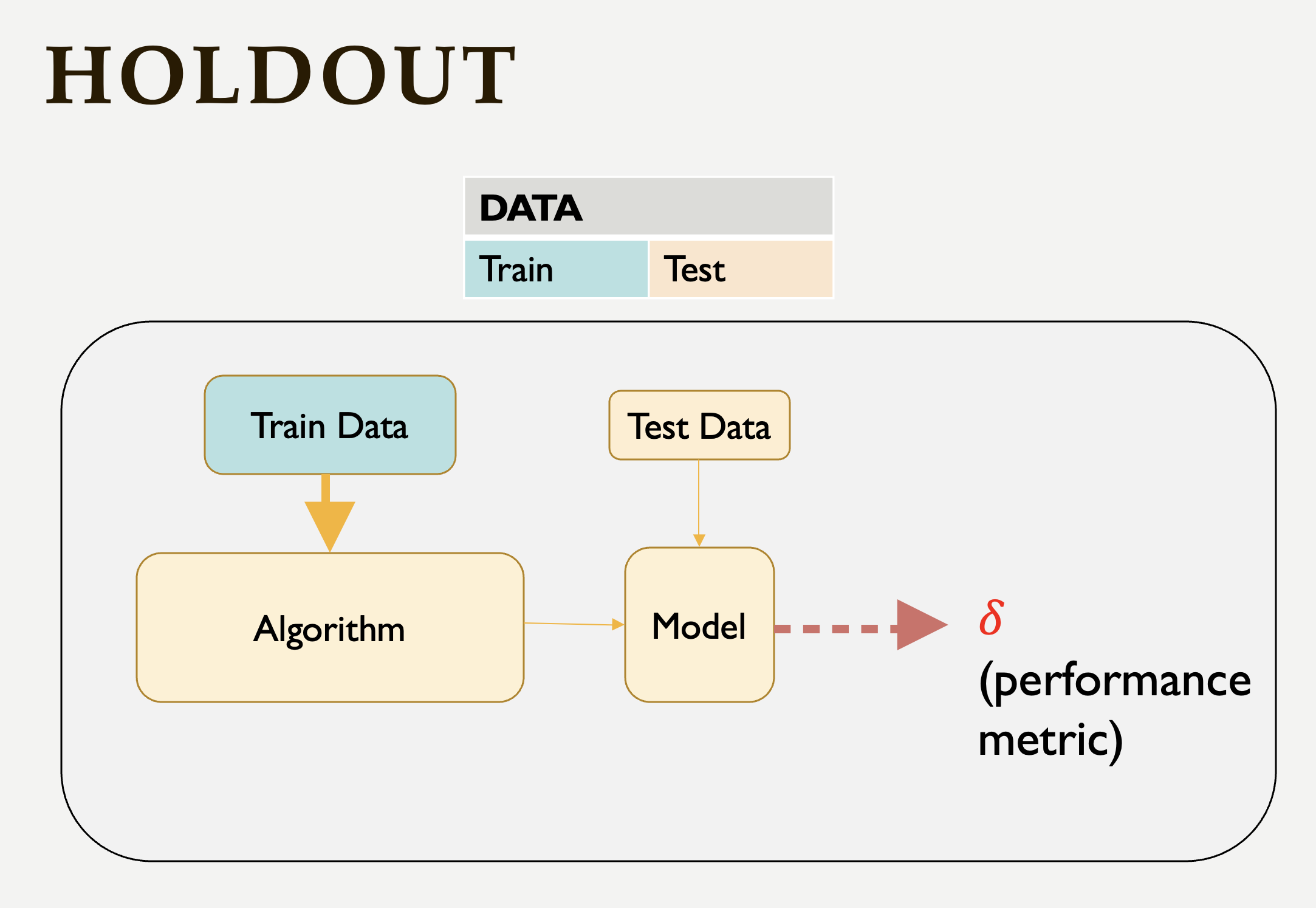
This schema says that each value of the hyperparameter generates one algorithm, and the train set is used to define parameters of interest of the algorithm. Then, test data is used to find the predictions. These predictions is used to find the model metrics which can be Mean Squared Error (MSE) in our example, since we run a regression model with a numeric target.

Deliverables

2.1. Split the data into train (80%) and test (20%).
2.2. Run the polynomial model from 1 to 5 degrees and calculate the Mean Squared Error value for each degree.
2.3. Plot each degree versus MSE and determine the degree of polynomial regression for your data.

Question 3 (2 points)

Since data splitting process is implemented randomly, the MSE values we obtain in regression (or the accuracy values in classification) will differ from one another. In this case, how do we decide which result to accept as the final outcome?

Although the literature provides various approaches to this problem, if we were all sitting around a table discussing possible solutions, we would likely consider averaging the MSEs (or any other metric such as accuracy, RMSE or $R^2$, etc.). Instead of relying on a single data split, repeating the process multiple times allows us to obtain more generalizable results and ensuring that the model performance metric is generalizable.

Determining the optimal train-test split ratio is another challenge that can be addressed using cross-validation. In the literature and many applications, we commonly see an 80% training and 20% test split. However, you can experiment with different ratios to observe how performance changes. A key consideration is that a large test set may introduce a pessimistic bias, while a small test set can lead to high variance. The plot below is an illustration from the Raschka’s paper using the Iris dataset to fit to KNN where $K$ is 3. You can see how accuracy changes when you change the train-test ratios. On the left plot, the ratio of test data is high (50%), and we cannot reach out that accuracy reported on the right hand side where the ratio of test is low (10%). For the low ratio of test data, we observe higher fluctuations on accuracy (high variance).

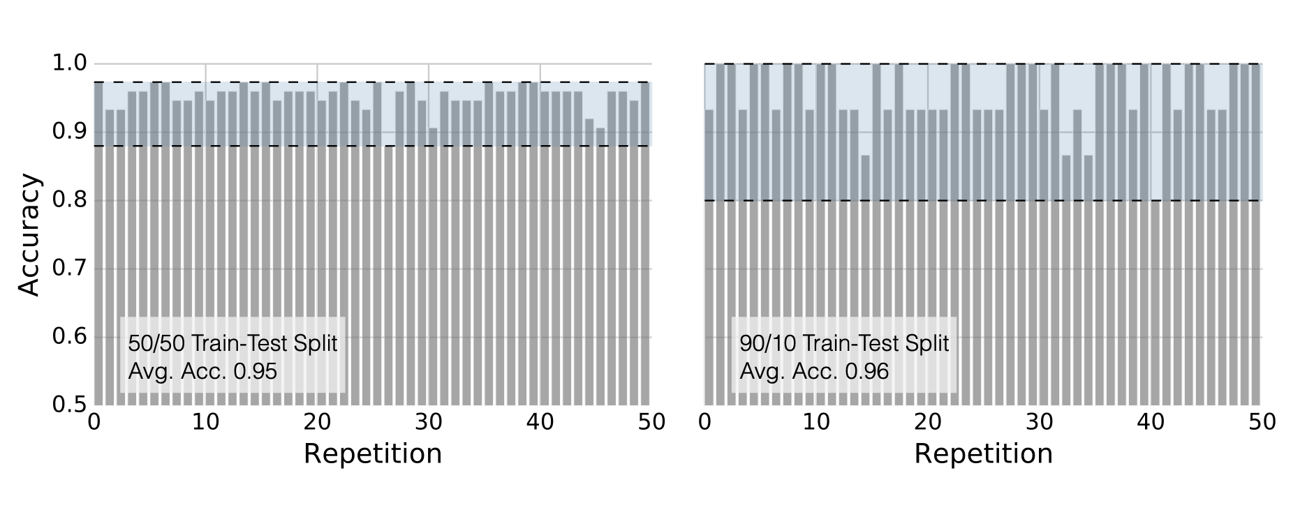
Image Source: Model Evaluation, Model Selection, and Algorithm Selection in Machine Learning, S. Raschka, arXiv:1811.1280v2, page.15, accessed Feb 28, 2025.

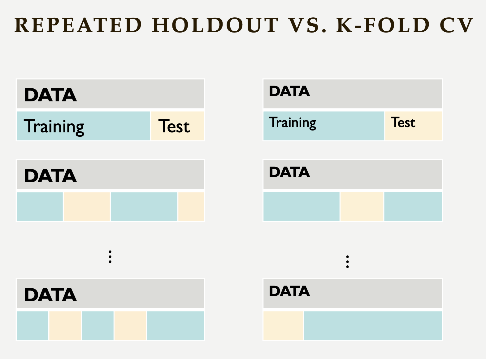
Repeated holdout and K-Fold cross-validation are both techniques for evaluating models by repeatedly splitting the data, but they differ in their approach. Repeated holdout randomly divides the dataset into training and test sets multiple times, averaging the results across iterations. However, this method can introduce bias since some data points may never be included in the test set, while others might appear multiple times. In contrast, K-Fold cross-validation systematically divides the dataset into K equal parts (folds), ensuring that each data point appears in the test set exactly once. This provides a more balanced evaluation and reduces the variability in performance estimates. Because of this, K-Fold cross-validation is generally preferred for a more reliable assessment of model performance. The following Figure illustrates their differences:

Figure 2. Holdout method

Deliverables

3.1. Repeat each step in Question 2 (2.1 and 2.2) for 100 times (use repeated holdout or K-fold cross-validation or both)
3.2. Plot randomly selected 10 processes
3.3. Find a generalizable MSE for this data.

Question 4 (2 points)

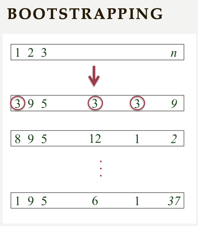
Another method used for cross-validation is bootstrapping, which was originally developed for other statistical purposes, primarily to estimate the sampling distribution of a statistic. However, it can also be adapted for cross-validation. Bootstrapping involves repeatedly sampling data with replacement to create multiple training datasets. Out-of-bag samples, those not selected for the bootstrap training set, are used as the test set. This allows us to estimate model performance across different subsets of data.

When you apply bootstrapping instead of repeated hold-out or cross-validation, the only difference in here from the previous example is that the sampling will be implemented with replacement. The following figure visually illustrates bootstrapping:

Deliverables

4.1. Repeat each step in Question 2 (2.1 and 2.2) for 100 times with bootstrapping sampling
4.2. Plot degree of polynomial versus MSE including all repeats and also mean MSE (bootstrap)
4.3. Did you notice any significant changes in your MSE values from Question 3.3 and bootstrapping?

Question 5 (2 points)

Classification methods are also required cross-validation to test prediction performances with some metrics such as accuracy. In this example, we will use Support Vector Machines (SVM) in scikit-learn to recognize images of hand-written digits from 0-9.

The following video give brief introduction to SVM:

The hand-written digits from 0-9 dataset consists of $8 \times 8$ pixel images of digits. The images attribute of the dataset stores $8 \times 8$ arrays of grayscale values for each image. There are 10 classes $~180$ samples per class. Total sample is 1797 with 64 dimensionality.

The Python code below include necessary libraries, how to load digits data and produce one example of the hand-written digits:

# Libraries
from sklearn.datasets import load_digits
from sklearn.svm import SVC
from sklearn.metrics import ConfusionMatrixDisplay, classification_report
from sklearn.model_selection import train_test_split
import matplotlib.pyplot as plt

# Load the Data
numbers = load_digits()
X = numbers.data
y = numbers.target

# Example
fig = plt.figure()
plt.imshow(numbers.images[0], cmap = plt.cm.binary)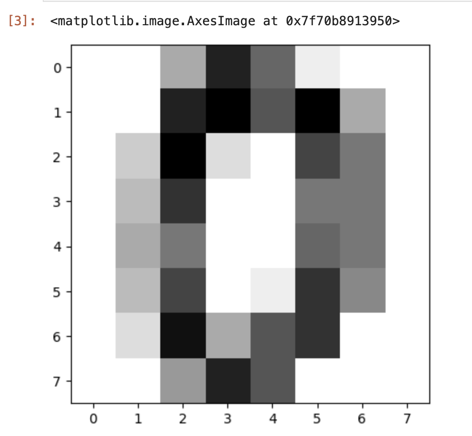

Figure 3. Example Hand-written Digit

This following line of code creates a SVM classifier using the SVC (Support Vector Classification) class from the sklearn.svm module.

svm = SVC(C=1, kernel='linear')

SVC initializes an SVM classifier, which is used for classification tasks.
The C parameter controls the trade-off between achieving a low error on the training data and maintaining a simple model. A higher C (e.g., C=10 or C=100) means the model will try to classify all training points correctly, even if that means creating a more complex decision boundary. A lower C (e.g., C=0.1) allows for more misclassified points but results in a simpler and more generalized model. Here, C=1 is a moderate choice that balances complexity and generalization.
kernel='linear' determines how the SVM transforms the data before finding a decision boundary. A linear kernel means the SVM will try to separate the classes using a straight line (or a hyperplane in higher dimensions) similar to the one showing in the video above. Other kernels like rbf (Radial Basis Function) and poly (Polynomial) allow for more flexible decision boundaries.

Also, SVM allows us to find classification report and confusion matrix in Python with the following code:

classification_report(y_test, predict_test) # predict_test contains the predicted class labels for the test dataset. It is generated by an SVM (or another classifier) using the .predict() function.

visual = ConfusionMatrixDisplay.from_estimator(svm, X_test, y_test)
visual.figure_.suptitle("Error matrix")
print('Error matrix:\n', visual.confusion_matrix)

When evaluating a machine learning model, a classification report is generated. In classification reports, you will see the following metrics. It has become one of the rare model output metrics that people (including me) working machine learning constantly sees but cannot remember their meanings :) You can always go back to this page or any page you find useful to see the meaning of those metrics.

Precision = TP / (TP + FP)

Measures how many of the predicted positives are actually correct. High precision means fewer false positives.

Recall = TP / (TP + FN)

Measures how many of the actual positives were correctly predicted. High recall means fewer false negatives.

F1 = 2 × (Precision × Recall) / (Precision + Recall)

Harmonic mean of precision and recall. A balanced measure, especially useful if there is an imbalance between precision and recall.

Support is the number of actual instances for each class in y_test. It tells us how many test samples belong to each class.

Deliverables

5.1. Use a SVM model to recognize handwritten digits (Divide the data: 80% for training the model, and 20% for testing the model).
5.2. After the model is trained, show the classification report and the confusion matrix
5.3. Explain what the confusion matrix tells us about the model’s performance.

Submitting your Work

Once you have completed the questions, save your Jupyter notebook. You can then download the notebook and submit it to Gradescope.

Items to submit

firstname_lastname_project1.ipynb

You must double check your .ipynb after submitting it in gradescope. A very common mistake is to assume that your .ipynb file has been rendered properly and contains your code, markdown, and code output even though it may not. Please take the time to double check your work. See here for instructions on how to double check this.

You will not receive full credit if your .ipynb file does not contain all of the information you expect it to, or if it does not render properly in Gradescope. Please ask a TA if you need help with this.