TDM 40100: Project 8 - Introduction to Time Series

Project Objectives

This project will introduce you to the essential steps of preparing time series data for analysis and forecasting. Time series data requires special attention during the cleaning and transformation process before applying any machine learning method. You will learn how to handle common challenges such as missing values and repeated timestamps to prepare data for modeling.

Learning Objectives

Understand the unique structure of time series data and why certain cleaning methods are required before analysis.
Identify and address common data quality issues such as missing values and duplicate timestamps.
Convert and format datetime variables using pandas.
Apply time based interpolation and feature transformation techniques to prepare data for time series analysis.
Gain experience in structuring raw weather data into a usable format for modeling or forecasting.

Use 4 cores for this project.

Dataset

The dataset is located at:

/anvil/projects/tdm/data/noaa_timeseries

If AI is used in any cases, such as for debugging, research, etc, we now require that you submit a link to the entire chat history. For example, if you used ChatGPT, there is an “Share” option in the conversation sidebar. Click on “Create Link” and please add the shareable link as a part of your citation.

The project template in the Examples Book now has a “Link to AI Chat History” section; please have this included in all your projects. If you did not use any AI tools, you may write “None”.

We allow using AI for learning purposes; however, all submitted materials (code, comments, and explanations) must all be your own work and in your own words. No content or ideas should be directly applied or copy pasted to your projects. Please refer to the-examples-book.com/projects/fall2025/syllabus#guidance-on-generative-ai. Failing to follow these guidelines is considered as academic dishonesty.

Introduction

“Climate is what we expect, weather is what we get.” – Mark Twain

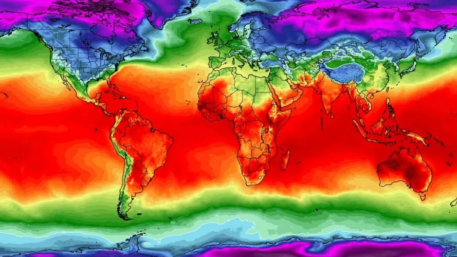
Figure 1. Global 2-meter air temperature anomalies on February 19, 2021, visualized by Climate Reanalyzer, Climate Change Institute, University of Maine.

Everyone is talking about climate change—but what does the data actually say? In this project, you will explore over 18 years of daily weather from Indianapolis and investigate how climate patterns are shifting over time. Of course, the data will not be a clean, pre-packaged dataset. Real data is messy. Some days are missing. Some values use symbols like "T" for trace amounts (small amounts close to 0) or "M" for missing entries. Before we can analyze trends or train a forecasting model, we will need to clean and prepare the data.

This dataset comes from National Oceanic and Atmospheric Administration (NOAA) Local Climatological Data and includes variables such as daily temperature, precipitation, humidity, wind speed, and snowfall for Indianapolis.

These are the key environmental indicators we will work with:

DailyAverageDryBulbTemperature: Average air temperature
DailyMaximumDryBulbTemperature and DailyMinimumDryBulbTemperature: Max and Min Air Temperature for the day
DailyPrecipitation: Rainfall or melted snow (inches)
DailyAverageRelativeHumidity: Moisture in the air
DailyAverageWindSpeed: Wind patterns (mph)
DailySnowfall: Snow accumulation (inches)

Why do we need to use time series analysis for this data?

Time series methods are specifically designed to work with data where observations are collected at consistent intervals—like daily, weekly, or monthly so we can understand how things change over time and make predictions about the future. This dataset is a good for time series analysis because it tracks temperature and other weather variables on a daily basis over 18+ years.

In this case, we’re interested in uncovering patterns in climate data, such as:

Seasonal trends (e.g., warmer summers, colder winters)
Long-term trends (e.g., gradual increase in temperature due to climate change),
Short-term fluctuations (e.g., sudden cold snaps or heatwaves),
And even forecasting future conditions based on past observations.

However, we cannot jump straight into modeling. Before building a time series model, we must ensure:

Dates are properly formatted and consistently spaced,
All variables are numeric and in usable units,
Missing or trace values (close to 0) are handled appropriately,
And the dataset contains no duplicated or skipped dates.

This project will guide you through these foundational steps. By the end, you will not only have a cleaned and structured dataset but you will also understand what makes time series unique, and how to prepare real-world data for powerful forecasting tools like ARIMA or LSTM neural networks.

Time series analysis is a crucial skill in data science, especially for applications in weather forecasting, finance, agriculture, and public health. Mastering the preparation process is your first step toward building models that can anticipate the future.

We will ask a series of questions to help you explore the dataset before the deliverables section. These are meant to guide your thinking. The deliverables listed under each question describe what you will need to submit.

Questions

Question 1 Explore One Year Worth of Data (2 points)

Before we clean or analyze anything, we need to take a step back and get to know the data. Your goal is to investigate what kind of time intervals the data uses and whether it’s ready for time series analysis.

Data Types

One important think to highlight is: data types matter. In time series analysis or any time you are plotting and cleaning your data, variables must be in the correct format to work properly. The DATE column needs to be stored as a datetime object so Python can recognize the order of events and perform date-based operations. Similarly, variables like temperature and precipitation must be numeric. If these are accidentally read as strings perhaps because of special characters your analysis may break or return misleading results. One of your first things you will need to do for question 1 is to inspect and confirm that each column had the correct data type before doing any deeper analysis.

The following are the standard or built-in data types in Python:

Numeric – int, float, complex
Sequence Type – str, list, tuple
Mapping Type – dict
Boolean – bool
Set Type – set, frozenset
Binary Types – bytes, bytearray, memoryview

Source from: www.geeksforgeeks.org/python-data-types/

Here are some additional questions to think about to help guide your exploration in question 1:

What kind of time intervals is the data in?
If we wanted our data to be on a daily level, is there something weird within the data that’s preventing that?
Are there duplicates for a given calendar day?
What kinds of variables and data types are currently included in the data? Which ones do you think will be useful for weather analysis?

To load the 2006 weather dataset, use the following code:

import pandas as pd
indy_climatedata_2006 = pd.read_csv("/anvil/projects/tdm/data/noaa_timeseries/indyclimatedata_2006.csv", low_memory=False)

Deliverables

1a. Load the 2006 weather dataset and preview the first few rows. Then, write 1–2 sentences describing any initial observations you notice in the data: are there patterns, missing values, or unusual entries?
1b. Check the number of rows and columns, and inspect the column names and data types. Output this information, then write 1–2 sentences explaining which columns seem most useful for daily weather analysis and whether the data types look appropriate.
1c. Convert the DATE column to datetime format using pd.to_datetime(). Output a few values from this column, then write 1–2 sentences noting what you observe: are there multiple observations per calendar day or anything unexpected?
1d. Count the number of unique calendar dates using .dt.date.nunique() and compare it to the total number of rows. Output these numbers, then write 1 sentence summarizing what this tells you about the structure of this dataset.

Question 2 Combine All Years (2 points)

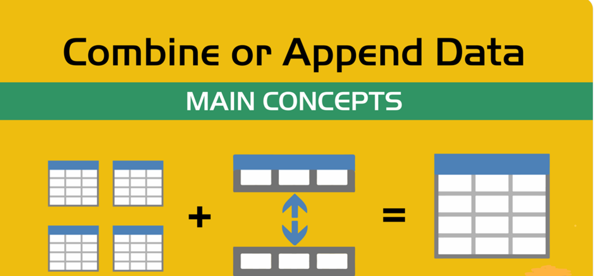
In many real-world projects, your data will not come clean in a tidy file. Instead, it will arrive across multiple files, years, or formats. It will often be like assembling a puzzle: each piece holds valuable information, but the full picture only comes into view once everything is combined neatly.

In our case, each year of daily weather observations is stored in its own file. Luckily, these files are consistent with each other because they share the same structure and the same column names. By stacking them together into a single, unified dataset, we are able to build a continuous timeline spanning nearly two decades of weather data.

By stacking these annual files together, we will be able to:

Track long-term climate trends in temperature, precipitation, snowfall, and more,
Detect seasonal patterns and anomalies across years,
Investigate how weather events are changing over time—key to studying climate change,
Prepare the data for meaningful time series analysis and modeling.

Our data files currently look like this:

indyclimatedata_2006.csv
indyclimatedata_2007.csv
indyclimatedata_2008.csv …
indyclimatedata_2024.csv

We can list them in ANVIL:

%%bash

ls /anvil/projects/tdm/data/noaa_timeseries/

Each file contains daily weather data for a single year—like the 2006 dataset. Our goal is to combine (or stack) these files into one continuous dataset so we can prepare it for time series analysis and explore long-term weather trends in Indianapolis.

You can think of it like stacking information — you’re placing one dataset on top of another. This process is often called appending or combining rows, and it’s how we build one larger dataset from many smaller ones with the same structure. Like in the image below:

Figure 2. Figure Source: “Combine or Append Data – Main Concepts,” The Power User, April 9, 2019.

After combining all years together ask yourself:

Are some years more complete than others?
What challenges might this pose for analysis?

Deliverables

2a. Stack the files from 2006–2024 into one DataFrame. You may use the function below to stack the data or write your own function:

import pandas as pd

def load_and_stack_climate_data(start_year=2006, end_year=2024, base_path="/anvil/projects/tdm/data/noaa_timeseries/"):
    dfs = []
    for year in range(start_year, end_year + 1):
        file_path = f"{base_path}indyclimatedata_{year}.csv"
        try:
            df = pd.read_csv(file_path, low_memory=False)
            df['year'] = year
            dfs.append(df)
        except FileNotFoundError:
            print(f"File not found for year {year}: {file_path}")
            continue
    combined_df = pd.concat(dfs, ignore_index=True)
    return combined_df

2b. Count the total number of rows in your combined dataset. Then, break it down by year: how many rows (or days) are recorded for each year? Output both the overall row count and the yearly breakdown.
2c. Use the code below to create a filtered version of your dataset that includes only the columns in columns_to_keep. Save this as a new DataFrame all_years_df_indy_climate.

columns_to_keep = ["DATE", "DailyAverageDryBulbTemperature", "DailyMaximumDryBulbTemperature", "DailyMinimumDryBulbTemperature", "DailyPrecipitation", "DailyAverageRelativeHumidity", "DailyAverageWindSpeed","DailySnowfall", "NAME"]

DF = DF[columns_to_keep]

2d. In 1–2 sentences, explain whether the new dataset is structured at a daily level. Based on what you see, are there multiple weather observations per day? What might you need to do to clean the data so that there’s only one row of weather data per calendar day?

Question 3 Clean Weather Data (2 points)

We’ll start by filtering the dataset to keep a small subset of variables that represent key daily weather conditions. These include average, minimum, and maximum temperatures, precipitation, humidity, wind speed, and snowfall.

Since we’re working with time series data, it’s important that the time variable follows a consistent interval such as daily, weekly, or monthly and that the values we’re analyzing over time are numeric. This structure allows us to properly visualize trends, build models, and interpret results. For this project, we’ll focus on preparing the data at the daily level.

As part of this preparation, you’ll notice that we’ll need to remove rows that are missing all weather measurements. These rows don’t provide any usable information and there’s nothing to visualize or analyze. However, we need to be careful not to include columns like DATE or NAME when removing rows. If we do, we might accidentally keep rows that only have a date or location but no actual weather data. Keeping those rows could result in misleading patterns, inaccurate summaries, or errors later in your analysis. These rows aren’t helpful for analysis, since they don’t contain any usable data. However, we don’t want to remove rows just because they include a date or station name we only want to drop rows where all of the selected weather columns are missing.

Deliverables

3a. Use the code below to drop any rows where all weather columns are missing, making sure to EXCLUDE "DATE" and "NAME" from the check. Then print the first 5 rows of the new DF.

# Create a list of weather-related columns to check
cols_to_check = [col for col in DF.columns if col not in ["DATE", "NAME"]]

# Drop rows where all weather columns are missing
DF = DF.dropna(subset=cols_to_check, how='all')

3b. Convert the DATE column in your dataframe to datetime format YYYY-MM-DD and preview the result to confirm it worked. (Hint: Use pd.to_datetime()).
3c. Print the shape of your cleaned dataset and display the range of dates it covers. (Hint: Use .min().date() and .max().date()).

Question 4 Prepare for Time Series Analysis (2 points)

Time series analysis requires data to be clean, numeric, and properly indexed by time. Before we can build models or create visualizations, we need to ensure our dataset is structured correctly.

Let’s walk through an example to see why this step matters.

Setting Date as Index and Interpolation

Suppose we try to interpolate (fill in) missing temperature values without setting the date as the index:

DF["DailyAverageDryBulbTemperature"].interpolate(method="time")

Running this will throw an error! The error will probably read something like "ValueError: time-weighted interpolation only works on Series or DataFrames with a DatetimeIndex."

Why? Because Python doesn’t know which column represents time. Time-based interpolation only works when the index is a datetime object.

Now, let’s fix that:

DF["DATE"] = pd.to_datetime(DF["DATE"]) # Ensure DATE is datetime format
DF = DF.set_index("DATE") # Set DATE as index
DF["DailyAverageDryBulbTemperature"].interpolate(method='time'), limit_direction='both')

This works! By setting DATE as the index, Python understands the data is time-ordered and can now interpolate gaps using the timeline.

Reset the Index

After setting the Date as Index, Python won’t recognize that it’s a normal column anymore. You can reset the index so DATE becomes a regular column again using DF.reset_index(inplace=True).

Trace Amounts

Next, let’s deal with another common problem in weather data: values like "T" that stand for trace amounts (small amount close to 0) of precipitation or snowfall. These aren’t numeric and could mess up our code.

For example, try converting a column like this to float:

DF["DailyPrecipitation"].astype(float)

You’ll get an error! It will probably read something like "ValueError: could not convert string to float: 'T'."

To fix this you can use .replace to replace the trace values with zero and .astype() to convert the trace values to a numeric value like this:

DF["DailyPrecipitation"] = DF["DailyPrecipitation"].replace("T", 0)
DF["DailyPrecipitation"] = DF["DailyPrecipitation"].astype(float)

Time series data is powerful but only if it’s properly structured. With consistent intervals on the x-axis (DATE) and numeric values on the y-axis (like temperature, precipitation, etc.), we can detect trends, spot anomalies, and build forecasting models.

Figure 3. Figure Source: Airbyte, 'What Is Time Series Data In Data Analysis (With Examples)', airbyte.com/data-engineering-resources/time-series-data

Deliverables

4a. Set the DATE column as the dataframe’s index. Then identify which columns are numeric by using .dtype().
4b. Use time-based interpolation to fill missing values in numeric columns. Hint: you can use .interpolate(method='time'), limit_direction='both')
4c. After interpolation, reset the index so DATE becomes a regular column again. Hint: you can use DF.reset_index(inplace=True).
4d. Find and replace any non-numeric "T" values in weather columns with 0 (e.g., precipitation, snowfall), convert the columns to float, and confirm no non-numeric values remain.

Question 5 Exploring Climate Trends Over Time (2 points)

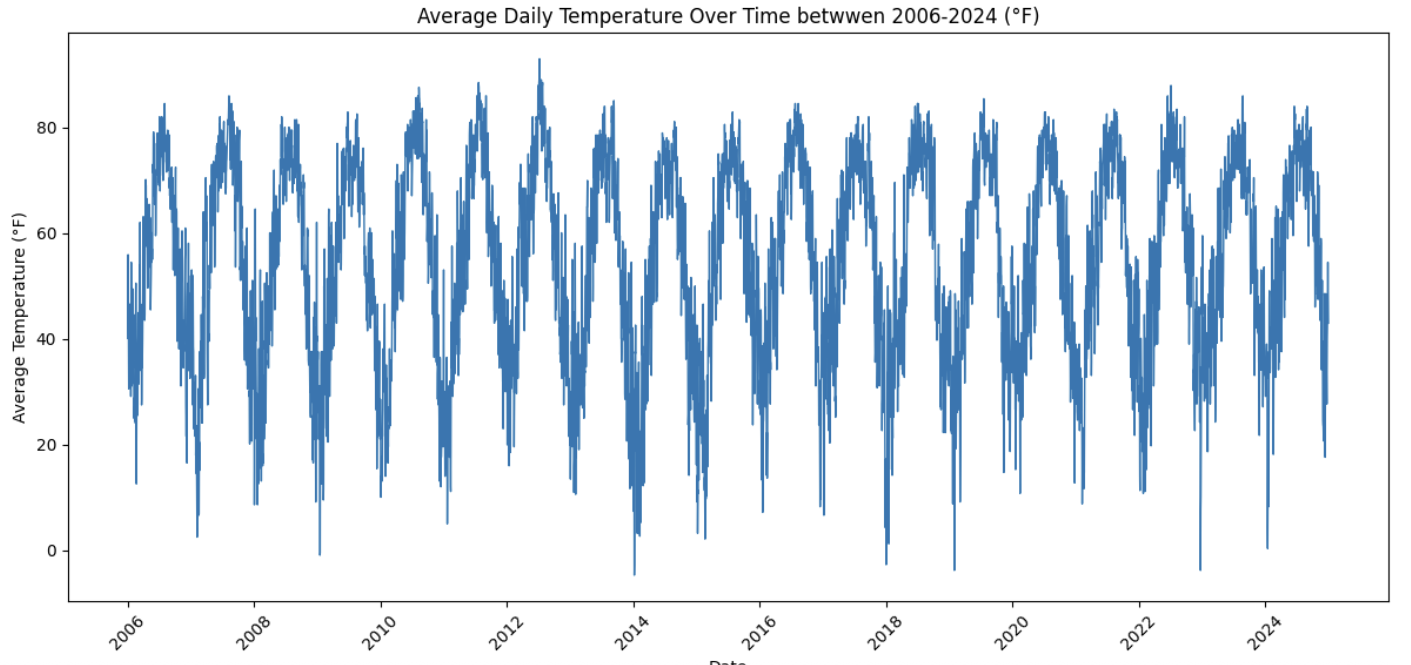
You’ve cleaned and prepared your data so now it’s time to visualize it. Try visualizing the full range of daily temperatures to uncover trends or shifts over the years. Then, focus on a single year. What patterns do you notice when you zoom in?

Deliverables

5a. Review your temperature column DailyAverageDryBulbTemperature. It is currently in Celcius. Convert it to Farenheit and name it DailyAverageDryBulbTemperature_Farenheit.
5b. Create a time series plot of daily average temperature DailyAverageDryBulbTemperature_Farenheit from 2006 to 2024. Write 1–2 sentences describing any trends you observe.

Hint: You can use the matplotlib library for plotting. A basic example might look like this (be sure to replace 'x' and 'y' with your actual column names):

import matplotlib.pyplot as plt
plt.plot(all_years_df_indy_climate['x'], all_years_df_indy_climate['y'], linewidth=1) # For YOU to Fill in

plt.title('Average Daily Temperature Over Time between 2006–2024 (°F)')
plt.xlabel('Date')
plt.ylabel('Average Temperature (°F)')

plt.xticks(rotation=45)
plt.tight_layout()
plt.show()

5c. Create a second plot for DailyAverageDryBulbTemperature_Farenheit focusing only on the year 2024. Then write 1-2 sentences on- what seasonal patterns or anomalies stand out?

Question 6 Create Time-Based Features (2 points)

Now that your dataset is clean and structured, you’re ready to extract new features from the date itself. In time series modeling, features like month, day of the year, or day of the week can help us detect patterns, capture seasonality, and build better forecasts.

For example:

Month can reveal seasonal trends—like hot summers or snowy winters.
Day of the week might help explain certain anomalies or weekly cycles.

Deliverables

6a. Add a new column to your dataset that captures the month (1–12) by extracting only the month from the DATE column. Ensure that this new column is a string.
6b. Now calculate the average temperature for each month by averaging across all years. Hint: You may want to use: .groupby('Month') and .mean().reset_index()
6c. Create a plot showing the average monthly temperatures across all years. What seasonal patterns or trends can you observe?

Submitting your Work

Once you have completed the questions, save your Jupyter notebook. You can then download the notebook and submit it to Gradescope.

Items to submit

firstname_lastname_project8.ipynb

You must double check your .ipynb after submitting it in gradescope. A very common mistake is to assume that your .ipynb file has been rendered properly and contains your code, markdown, and code output even though it may not. Please take the time to double check your work. See here for instructions on how to double check this.

You will not receive full credit if your .ipynb file does not contain all of the information you expect it to, or if it does not render properly in Gradescope. Please ask a TA if you need help with this.