TDM 40200: Project 5 - Introduction to MLOps - Extended

Last project we made it a point to organize our methods into their own files like for data loading and for training, etc. This is pretty standard, and because of what we did last project, the conversion to another great method will be very simple. One of the most important things, especially as projects grow, is encapsulation. It reduces risks and confusion, separates concerns, etc.

We are going to introduce PyTorch Lighting which can help with this. It does not necessarily abstract all your code but it helps organize your model instantiation, training loops, hyperparameters and more in a very intuitive object oriented way.

First things first, we will focus on creating a LightningModule for our current PyTorch model - with this we can define some standard operations and more easily scale our operation.

Please create a new file called lightning.py in the src/ directory.

Here, we are going to create a class that inherits from pl.LightningModule and then we will define our model, loss function, and optimizer. We will also define a much simpler looking training loop.

Here we define how our model class will be initialized. It inherits pl.LightningModule which allows our instantiation to make use of the parent class’s functions, attributes, features, etc. (the parent class being pl.LightningModule).

If that is a little hazy, take this for example:

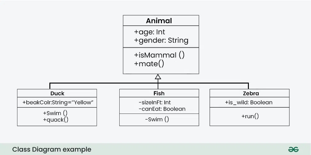
Here we see Duck, Fish and Zebra. They are all animals and fundamentally have a set of similar attributes, so you can create a parent class with a minimum set of attributes that all animals have and then have each animal inherit from it. This way you can ensure some baseline functionality for all animals like age, gender, +isMammal(), etc. They can also each have their own unique features like +swim(), +fly(), +run(), etc.

Also, parent classes will sometimes leave functions blank and expect you to fill them in i.e. all animals mate but they do not all have the same mating behavior, hence you may need to override it when creating a Duck vs creating a Fish.

In our case, WineQualityClassifier (Duck, Fish, Zebra etc.) inherits from pl.LightningModule (Animal) and inherits the features and attributes of the parent class like forward, training_step, configure_optimizers, etc. It can also have its own unique features like model, loss_fn, etc.

But remember how we already created a model class in the previous project? We can use that here to pass in as a parameter to our WineQualityClassifier class. This way we can make our lightning module more flexible and reusable.

Moving on, we can then define other key methods we will want in our model class:

All three of these are keyword functions we need to implement in our subclass since these are core to the function of our model:

By defining these methods in the LightningModule class, they are automatically called when the model is trained and validated.

If you noticed from last project, we did not define a validation step, only a training and test step, but here we can easily add one by defining a validation_step method. This will also be automatically run during training time.

Note that validation is used to fine tune hyperparameters and assess current performance but is not actually trained on.

Comparing with last project, the overall steps are very similar but instead we use the pl.LightningModule class to help us organize our logic. It is much easier and cleaner to define the steps for your model using this method. It will also remove the need to define the training loops like we have in src/trainer.py since we have it all within the one class. Nice and convenient!

Now that we have defined our custom model using LightningModule, we can import it in the main.py file just like how we did with the previous project’s model:

Note that in the current state, our pipeline in main.py will not work properly without some modification. Since we are using this approach, the training for our model relies on a slightly different form of the dataloader which we will touch on in the next question. We will also work on integrating everything in Question 4.

Last project we had this setup:

It is already fairly clean and makes use of the helper functions we defined last time, but these steps are pretty much the same everywhere so there is no reason to have them in our main logic. We already create a dataloader here in our helper functions:

But instead of having multiple helper functions in our main logic to eventually get to a dataloader, we can use the datamodule provided by Lightning instead - LightningDataModule. We once again create a custom class that inherits from a module and implements the relevant functions. This encapsulates a lot of the core boiler plate repeated logic into a nice class.

Open up data_loader.py and we will essentially just wrap these functions we already created into the DataModule object. Since we are using a LightningDataModule, we need to implement the following methods:

However we first need to quickly talk about the data we are using. This dataset consists of 11 features and 1 target label column quality. In your notebook please load the data and print the first few rows to see what it looks like.

We see there is a column called type which is either Red or White but we want to predict the quality of the wine based on the other features, so we will drop the type column.

So we just need to make a slight modification to how we obtain our X and y variables in our setup method.

Please fill in the …​ with the appropriate code (which is the same logic from our helper functions in the previous project) but this time please use the attributes we defined in the init method when encoding and splitting the data (i.e. self.data_path, self.batch_size, self.train_split)

Since our logic is now encapsulated, you can delete those helper functions we created last time.

Before we move on, we are going to add a quick data transformation into our datamodule to our target labels. Originally, the quality is rated between 0 to 10 which is a lot classes and the rating is somewhat subjective, so how can our model accurately differentiate between a 6 and a 7? To get around this, we are going to 'bin' the quality scores into 3 categories. This way, its less granular and more manageable for our model leading to some more interpretable results.

Please modify the setup method to include this:

Now that we have our datamodule class setup, we can remove those helper function calls we have in our main.py file since we have it all encapsulated in our LightningDataModule class. There now remains only one thing to do before we can test our pipeline!

If you remember last project we decided to create those helper functions like train_one_epoch to hide the nitty gritty details like zero the gradient. We can use the Trainer method from PyTorchLightning to do all that, but even cleaner. Our main.py should now look like this:

It abstracts all those annoying little details and makes use of your simple training_step in your LightningModule class to perform training to your specifications. It also has a bunch of different parameters you can pass into it to customize your training - we will touch on a couple later.

Nice! Now we have a pretty sick streamlined training setup. But, we have all those model and training parameters we are specifying when instantiating our classifiers and datamodules, we can use a different approach to manage them. We put everything into the config.py last time - path variables, model parameters, etc. We are going to move those model parameters into a YAML file called model.yaml. YAML files are similar to JSON in the sense they allow us to create a more readable and structured format for our configurations. We will also do a quick intro to a commonly used library called Pydantic which helps us validate schemas - this is to just make sure we are not attempting to load malformed data into our model.

Since we are creating more and more configuration type files, why do not we first create a new directory called config/ at the root level (at the same level as src, notebooks etc.). Move config.py into it and then create a model.yaml file in that directory.

The new file structure should resemble this:

This is the same information we had in our config.py (changed the EPOCHS variable to 5 for faster training), but in YAML format - it is very similar to JSON if you are familiar and is very often used for specifying configs.

Okay, so we now have a new streamlined training setup, a new config directory and we have moved our configurations for our model into a new YAML file. Now, we want to actually use the configurations we specified in our YAML file which in it of itself is very simple and can be done like so:

But note that this does not check the formatting of our YAML. What if there is some malformed configuration or a malicious configuration? We can enforce some safety using a library called Pydantic.

So in a new file called validation.py under our config directory, we are going to use Pydantic to define schemas for how our data should look. Pydantic does this by using Python classes with specified attributes and datatypes (more examples in their docs).

Here is an example of how we can define a schema for our training and model configurations:

This creates a class for the training and model parameters which contain their respective attributes and datatypes. When a single class uses both of these as types for the training and model attributes, those attributes should be defined in the configuration file. The load_config() returns you an object that contains all the parameters needed. This is good because you can experiment with different model and training parameters and just need to change the file paths being loaded in!

This is very nicely abstracted so now wherever we need to get our model parameters, we can load them in like so:

So now, in main.py we could replace all references to things like TRAIN_SPLIT with

But we can take this one step further…​

Instead of passing every training parameter through main.py, we can use a pretty slick feature of class inheritance to load config values behind the scenes for both WineQualityClassifier and WineQualityDataModule.

We are going to add a function to both called from_config_path with a special decorator @classmethod (more info can be found at classmethod(), Python document). The datamodule version takes config_path and data_path, while the classifier version takes model and config_path.

We will call the `load_config() function in both files (meaning you need import it there, too), and return an instance of the class:

This way we can pull training parameters from YAML while still passing the instantiated neural network into the classifier, which keeps the model definition and Lightning training logic cleanly separated.

Inside your notebook, please try loading the configs successfully and then changing a value in the model.yaml that would break and see the output:

Now let’s integrate everything we have built!

Alot of the work is now performed in the classes themselves and in the from_config_path methods which validates the configurations for us and then instantiates the classes. This way we can update our main.py to a much cleaner look:

Lets run our new pipeline! First though, we should comment out the old code to graph and save model weights since we are not using them anymore. However, we still need to save the label encoder so we can use it when serving the model, please go into the src/data_loader.py file and add the following code to the end of the setup() function:

Now we should be able to run our new pipeline! Quick check, our main.py should now look like this:

In your notebook, please run this code to see the validation results:

The output looks a little cluttered because of all the CUDA / TensorFlow warnings about not running in a GPU environment printed at startup but you can safely ignore them.

Also note that in the same directory level as intro_mlops_2 you should see a new directory called lightning_logs/ with a subdirectory called version_X/ containing the training logs.

Each version contains a events.out.tfevents file which is the training log. You can normally view the training logs by using something like TensorBoard but it will not quite work in Anvil so we will look at a different way to view the logs. Each version folder also contains a hparams.yaml file which contains the hyperparameters used for that version of the training as well as a checkpoints/ folder which contains the checkpoint files for that version of the training. For now, please just run this command to show your lightning logs:

Now let’s enhance our training with some useful callbacks.

In PyTorch Lightning, a callback is a small piece of logic that "hooks into" the training process at the right time (end of an epoch, after validation, when saving checkpoints, etc.). Instead of writing extra if statements and bookkeeping code in your training loop, you instantiate a callback object and attach it to the Trainer object which then runs the callbacks for you at the appropriate times!

Callbacks are definitely worth learning because they are one of the most common ways to make training:
- safer → avoid overfitting / wasted compute
- more reproducible → automatically save the best model
- more scalable → easy to add more behaviors later without rewriting your model code

Just to confirm lets see the contents of our logs/ directory:

MLflow is widely used in industry for experiment tracking, model registry, and deployment. Last question we integrated our Lightning module with our config files and callbacks and even adding some custom logging to a CSV file. Here we are going to implement a more robust logging solution using MLflow. We will log parameters, metrics, and the trained model so every run is reproducible and easy to compare.

Getting it set up is actually really simple. All you need to do is wrap your existing training in an MLflow run. By default MLflow saves runs under mlruns/ in the current directory (you can set MLFLOW_TRACKING_URI to use a different location).

You can remove the old logic that used the CSVLogger and printed to the console or wrote results.log or saved only weights with torch.save, since MLflow now stores the full model and metrics for each run.

If your environment allows it, you can run mlflow ui in a terminal to open a local web UI and compare runs visually but in restricted environments (like on Anvil) you typically cannot open a server but you can still inspect runs programmatically (using Python code/API calls instead of a browser).

We will put all of that logic in a file called see_runs.py in your src/ folder. The file loads the runs, prints the table, plots val_loss and val_accuracy, and prints the best run. From your notebook you just call one function; you do not run any of the plotting or MLflow code in the notebook. Below is the full code that goes in the file, then we break it down into parts.

Last project we created a basic API using FastAPI to serve a prediction — but we skipped a critical step which is setting up input schema validation. This is essential for any API whether it is public or internal. It ensures you will not be sending malformed data into your model which can cause the model to fail outright, but the real danger are silent errors. Silent errors in this case would be when the API does not throw an error, the model returns a prediction, but the prediction is entirely incorrect. This is much worse because it can be hard to detect and someone could take action based on the wrong prediction. Rigorous validation helps defend against these risks.