TDM 40200: Project 11 - Large Language Models (LLMs): Word Embeddings
Project Objectives
This project will focus on the concept of word embeddings, or different ways to represent words other than simply using the word itself. We will explore many different methods of representing words, such as one-hot encoding, bag of words, and word2vec. We will also look at ways to compare word embeddings, such as distance and cosine similarity.
Questions
Question 1 (2 points)
In this project, we will be learning about word embeddings and how they are used. Word embeddings, simply put, are ways to embed words into a vector space. This allows us to represent words in a way that can capture their meaning, context, relationships with other words, etc. There are many different algorithms for creating word embeddings, and we will be looking at a few of them in this project. After we look at algorithms for representing words, we will look at algorithms to compare these word embeddings. We will also look at how to visualize word embeddings.
Gensim is a Python library for natural language processing that has many different algorithms for creating word embeddings. Originally, this library was created to help address limitations in practical applications of representing large text collections in vector space, particularly memory and speed. The Gensim publication Software for Topic Modeling with Large Corpora describes these limitations and how Gensim addresses them. The library is open source and can be found at github.com/piskvorky/gensim.
To start, please copy in your read_lines and clean_text functions from last project to start. We need these to read in the data and clean it up before it can be used.
The first form of word embedding we will look at is one-hot encoding. If you remember from last semester’s machine learning projects, one-hot encoding is a way to represent categorical variables as binary vectors. As a refresher, we could turn categorical labels into integers with a process known as label encoding, but this can create problems with non-ordinal data being seen as ordinal (i.e., the numbers 1,2,3 seen as having a relationship when they should not). One-hot encoding solves this problem by creating a binary vector for each category. For example, if we have three categories: apple, banana, orange, we could represent them as follows:
-
apple: [1, 0, 0]
-
banana: [0, 1, 0]
-
orange: [0, 0, 1]
This allows us to represent categorical variables without creating false ordinal relationships. Please create your own one_hot_encoding function that takes in a list of words and returns a list of one-hot encoded vectors. You can use the numpy library to help with this.
In short, you should count how many unique words are input to the function, create a list of zeros of that length, and then set the index of that word to 1. For example, if the input is ["apple", "banana", "orange"], the output should be:
[ [1, 0, 0], [0, 1, 0], [0, 0, 1] ]
Here is the function outline to help you get started:
def one_hot_encoding(words):
    # Create a list of unique words
    # your code here

    # Create an empty list of one-hot encoded vectors
    # your code here

    # Loop through the words and create the one-hot encoded vectors
    for i, word in enumerate(words):
        # Create a list of zeros of the same length as the number of unique words
        # your code here

        # Set the value in the vector to 1 at the index of the word
        # your code here

        # Append the vector to the list of one-hot encoded vectors
        # your code here

    # return the list of one-hot encoded vectors
    # your code here
And here are some test cases to help you get started:
print(one_hot_encoding(clean_text(' '.join(read_lines('/anvil/projects/tdm/data/amazon/music.txt', 2, 100))).split()))
# should output the following:
'''
[[0, 0, 0, 0, 0, 1, 0, 0, 0, 0, 0, 0, 0, 0, 0, 0, 0, 0, 0, 0, 0, 0, 0], [0, 0, 0, 0, 0, 0, 0, 0, 0, 0, 0, 1, 0, 0, 0, 0, 0, 0, 0, 0, 0, 0, 0], [0, 0, 0, 0, 0, 0, 0, 0, 1, 0, 0, 0, 0, 0, 0, 0, 0, 0, 0, 0, 0, 0, 0], [0, 0, 0, 0, 0, 0, 0, 0, 0, 1, 0, 0, 0, 0, 0, 0, 0, 0, 0, 0, 0, 0, 0], [1, 0, 0, 0, 0, 0, 0, 0, 0, 0, 0, 0, 0, 0, 0, 0, 0, 0, 0, 0, 0, 0, 0], [0, 0, 0, 0, 0, 0, 0, 0, 0, 0, 0, 0, 1, 0, 0, 0, 0, 0, 0, 0, 0, 0, 0], [0, 0, 0, 0, 0, 0, 0, 0, 0, 0, 0, 0, 0, 0, 0, 0, 0, 1, 0, 0, 0, 0, 0], [0, 0, 0, 0, 0, 0, 0, 0, 0, 0, 0, 0, 0, 0, 0, 1, 0, 0, 0, 0, 0, 0, 0], [0, 0, 0, 1, 0, 0, 0, 0, 0, 0, 0, 0, 0, 0, 0, 0, 0, 0, 0, 0, 0, 0, 0], [0, 0, 0, 0, 1, 0, 0, 0, 0, 0, 0, 0, 0, 0, 0, 0, 0, 0, 0, 0, 0, 0, 0], [0, 0, 0, 0, 0, 0, 0, 0, 0, 0, 0, 0, 0, 0, 0, 0, 0, 0, 1, 0, 0, 0, 0], [0, 0, 0, 0, 0, 0, 0, 0, 0, 0, 0, 0, 0, 0, 0, 0, 0, 0, 0, 0, 0, 0, 1], [0, 0, 0, 0, 0, 0, 0, 0, 0, 0, 0, 0, 0, 0, 0, 0, 1, 0, 0, 0, 0, 0, 0], [0, 1, 0, 0, 0, 0, 0, 0, 0, 0, 0, 0, 0, 0, 0, 0, 0, 0, 0, 0, 0, 0, 0], [0, 0, 0, 0, 0, 0, 0, 1, 0, 0, 0, 0, 0, 0, 0, 0, 0, 0, 0, 0, 0, 0, 0], [0, 0, 0, 0, 0, 0, 0, 0, 0, 0, 0, 0, 0, 0, 1, 0, 0, 0, 0, 0, 0, 0, 0], [0, 0, 0, 0, 0, 0, 0, 0, 0, 0, 0, 0, 0, 0, 0, 0, 0, 0, 0, 0, 1, 0, 0], [0, 0, 0, 0, 0, 0, 0, 0, 0, 0, 0, 0, 0, 0, 0, 0, 0, 0, 0, 1, 0, 0, 0], [0, 0, 0, 0, 0, 0, 0, 0, 0, 0, 0, 0, 0, 0, 0, 0, 0, 0, 0, 0, 0, 1, 0], [0, 0, 0, 0, 0, 0, 0, 0, 0, 0, 0, 0, 1, 0, 0, 0, 0, 0, 0, 0, 0, 0, 0], [0, 0, 0, 0, 0, 0, 0, 0, 0, 0, 1, 0, 0, 0, 0, 0, 0, 0, 0, 0, 0, 0, 0], [0, 0, 1, 0, 0, 0, 0, 0, 0, 0, 0, 0, 0, 0, 0, 0, 0, 0, 0, 0, 0, 0, 0], [0, 0, 0, 0, 0, 0, 1, 0, 0, 0, 0, 0, 0, 0, 0, 0, 0, 0, 0, 0, 0, 0, 0], [0, 0, 0, 0, 0, 0, 0, 0, 0, 0, 0, 0, 0, 1, 0, 0, 0, 0, 0, 0, 0, 0, 0]]
'''

print(one_hot_encoding(clean_text(' '.join(read_lines('/anvil/projects/tdm/data/amazon/music.txt', 1, 210))).split()))
# should output the following:
'''
[[1, 0, 0, 0, 0, 0, 0, 0, 0, 0, 0, 0, 0, 0, 0, 0, 0, 0, 0, 0, 0, 0, 0, 0, 0, 0, 0], [0, 0, 0, 0, 0, 0, 0, 0, 0, 1, 0, 0, 0, 0, 0, 0, 0, 0, 0, 0, 0, 0, 0, 0, 0, 0, 0], [0, 0, 0, 0, 0, 0, 0, 0, 0, 0, 0, 0, 1, 0, 0, 0, 0, 0, 0, 0, 0, 0, 0, 0, 0, 0, 0], [0, 0, 1, 0, 0, 0, 0, 0, 0, 0, 0, 0, 0, 0, 0, 0, 0, 0, 0, 0, 0, 0, 0, 0, 0, 0, 0], [0, 0, 0, 0, 0, 0, 0, 0, 0, 0, 0, 0, 0, 0, 0, 0, 0, 0, 0, 0, 0, 0, 0, 0, 1, 0, 0], [0, 0, 0, 0, 0, 0, 0, 0, 0, 0, 0, 0, 0, 0, 0, 1, 0, 0, 0, 0, 0, 0, 0, 0, 0, 0, 0], [0, 0, 0, 0, 0, 0, 0, 0, 0, 0, 0, 0, 0, 0, 0, 0, 1, 0, 0, 0, 0, 0, 0, 0, 0, 0, 0], [0, 0, 0, 0, 0, 0, 0, 0, 0, 0, 0, 0, 0, 0, 0, 1, 0, 0, 0, 0, 0, 0, 0, 0, 0, 0, 0], [0, 0, 0, 0, 0, 0, 0, 0, 0, 0, 0, 0, 0, 1, 0, 0, 0, 0, 0, 0, 0, 0, 0, 0, 0, 0, 0], [0, 0, 0, 0, 0, 0, 0, 0, 0, 0, 0, 0, 0, 0, 0, 0, 0, 1, 0, 0, 0, 0, 0, 0, 0, 0, 0], [0, 0, 0, 0, 0, 0, 0, 0, 0, 0, 0, 1, 0, 0, 0, 0, 0, 0, 0, 0, 0, 0, 0, 0, 0, 0, 0], [0, 0, 0, 0, 0, 0, 0, 1, 0, 0, 0, 0, 0, 0, 0, 0, 0, 0, 0, 0, 0, 0, 0, 0, 0, 0, 0], [0, 0, 0, 0, 0, 0, 0, 0, 0, 0, 1, 0, 0, 0, 0, 0, 0, 0, 0, 0, 0, 0, 0, 0, 0, 0, 0], [0, 0, 0, 0, 0, 0, 0, 0, 0, 0, 0, 0, 1, 0, 0, 0, 0, 0, 0, 0, 0, 0, 0, 0, 0, 0, 0], [0, 0, 0, 0, 0, 0, 0, 0, 1, 0, 0, 0, 0, 0, 0, 0, 0, 0, 0, 0, 0, 0, 0, 0, 0, 0, 0], [0, 0, 0, 0, 0, 0, 0, 0, 0, 0, 0, 0, 0, 0, 0, 0, 0, 0, 0, 1, 0, 0, 0, 0, 0, 0, 0], [0, 0, 0, 0, 0, 0, 0, 0, 0, 1, 0, 0, 0, 0, 0, 0, 0, 0, 0, 0, 0, 0, 0, 0, 0, 0, 0], [0, 0, 0, 0, 1, 0, 0, 0, 0, 0, 0, 0, 0, 0, 0, 0, 0, 0, 0, 0, 0, 0, 0, 0, 0, 0, 0], [0, 0, 0, 0, 0, 0, 0, 0, 0, 0, 0, 0, 0, 0, 0, 0, 0, 0, 1, 0, 0, 0, 0, 0, 0, 0, 0], [0, 0, 0, 0, 0, 0, 0, 1, 0, 0, 0, 0, 0, 0, 0, 0, 0, 0, 0, 0, 0, 0, 0, 0, 0, 0, 0], [0, 0, 0, 0, 0, 0, 0, 0, 0, 0, 0, 0, 0, 0, 0, 0, 0, 0, 0, 0, 0, 1, 0, 0, 0, 0, 0], [0, 0, 0, 0, 0, 0, 0, 0, 0, 0, 0, 0, 0, 1, 0, 0, 0, 0, 0, 0, 0, 0, 0, 0, 0, 0, 0], [0, 0, 0, 0, 0, 0, 0, 0, 0, 0, 0, 0, 0, 0, 0, 0, 0, 0, 0, 0, 0, 0, 0, 1, 0, 0, 0], [1, 0, 0, 0, 0, 0, 0, 0, 0, 0, 0, 0, 0, 0, 0, 0, 0, 0, 0, 0, 0, 0, 0, 0, 0, 0, 0], [0, 0, 0, 0, 0, 0, 0, 0, 0, 0, 0, 0, 0, 0, 0, 0, 0, 0, 0, 0, 1, 0, 0, 0, 0, 0, 0], [0, 0, 0, 0, 0, 0, 0, 0, 0, 0, 0, 0, 0, 0, 0, 0, 0, 0, 0, 0, 0, 0, 1, 0, 0, 0, 0], [0, 0, 0, 0, 0, 0, 0, 0, 0, 0, 0, 0, 0, 0, 0, 0, 0, 0, 0, 0, 0, 0, 0, 0, 0, 0, 1], [0, 0, 0, 0, 0, 0, 0, 0, 0, 0, 0, 0, 0, 0, 1, 0, 0, 0, 0, 0, 0, 0, 0, 0, 0, 0, 0], [0, 0, 0, 0, 0, 0, 1, 0, 0, 0, 0, 0, 0, 0, 0, 0, 0, 0, 0, 0, 0, 0, 0, 0, 0, 0, 0], [0, 0, 0, 0, 0, 0, 0, 0, 0, 0, 0, 0, 0, 0, 0, 1, 0, 0, 0, 0, 0, 0, 0, 0, 0, 0, 0], [0, 0, 0, 0, 0, 0, 0, 0, 0, 0, 0, 0, 0, 0, 0, 0, 0, 0, 0, 0, 0, 0, 0, 0, 0, 1, 0], [0, 0, 0, 1, 0, 0, 0, 0, 0, 0, 0, 0, 0, 0, 0, 0, 0, 0, 0, 0, 0, 0, 0, 0, 0, 0, 0], [0, 0, 0, 0, 0, 1, 0, 0, 0, 0, 0, 0, 0, 0, 0, 0, 0, 0, 0, 0, 0, 0, 0, 0, 0, 0, 0], [0, 1, 0, 0, 0, 0, 0, 0, 0, 0, 0, 0, 0, 0, 0, 0, 0, 0, 0, 0, 0, 0, 0, 0, 0, 0, 0]]
'''
Based on these outputs, do you think it is practical to use one-hot encoding for word embeddings? Why or why not? (hint: Imagine we have a document with 100000 unique words)
Clearly, one-hot encoding is not a practical way to represent words for large datasets. It contains very little information about the words themselves, and takes up an extraordinary amount of space. The next option we can look at is a bag of words model. Bag of words is very easy conceptually. It is simply a dictionary of words and their counts. For example, if we have the following text:
"I like to eat apples and bananas. I like to eat oranges."
We could represent this using bag of words as:
{ "I": 2, "like": 2, "to": 2, "eat": 2, "apples": 1, "and": 1, "bananas": 1, "oranges": 1 }
This is a much more compact representation of the text, and it also maintains the basic information of the words themselves. The bag of words model is a very simple way to represent text, and it is often used as a baseline for more complex models.
Please implement a bag_of_words function that takes in a list of words and returns a dictionary of word counts. You can use the collections library to help with this.
def bag_of_words(words):
    # Create a dictionary of word counts
    # your code here

    # Return the dictionary of word counts
# your code here|
HINT: The |
And, here are the same test cases as before, using the bag_of_words function:
print(bag_of_words(clean_text(' '.join(read_lines('/anvil/projects/tdm/data/amazon/music.txt', 2, 100))).split()))

# should return the following:
'''
{'pretty': 1, 'good': 1, 'this': 1, 'is': 1, 'one': 1, 'of': 2, 'my': 1, 'favorite': 1, 'cds': 1, 'ive': 1, 'seen': 1, 'transsiberian': 1, 'orchestra': 1, 'three': 1, 'times': 1, 'and': 1, 'loved': 1, 'every': 1, 'minute': 1, 'it': 1, 'they': 1, 'are': 1, 'awesome': 1}
'''

print(bag_of_words(clean_text(' '.join(read_lines('/anvil/projects/tdm/data/amazon/music.txt', 1, 210))).split()))
# should return the following:
'''
{'great': 2, 'musicianship': 2, 'this': 2, 'one': 1, 'has': 1, 'it': 3, 'all': 1, 'is': 2, 'so': 1, 'refreshing': 1, 'to': 2, 'hear': 1, 'level': 1, 'of': 1, 'especially': 1, 'compared': 1, 'what': 1, 'considered': 1, 'on': 1, 'the': 1, 'radio': 1, 'these': 1, 'daysbuy': 1, 'you': 1, 'wont': 1, 'be': 1, 'disappointed': 1}
'''-
Implement the
one_hot_encodingfunction and test it with the provided test cases. -
Answer the question about the practicality of one-hot encoding for word embeddings.
-
Implement the
bag_of_wordsfunction and test it with the provided test cases.
Question 2 (2 points)
Bag of words is helpful, but still has its limitations. For instance, it does not maintain the order/context of the words. For example, "The dog chases the squirrel" and "The squirrel chases the dog" would be represented the same way, although they have fundamentally different meanings. This is where word2vec comes in. Word2vec is a more advanced algorithm for creating word embeddings that takes into account the context of the words. It uses a neural network to learn the relationships between words in a corpus, and can create dense vector representations of words that capture their meaning and context. Luckily for you, we don’t need to go through the trouble of implementing this ourselves. Gensim has a built-in function for this that is built on top of Fortran and C bindings to ensure that it is extremely fast and efficient. The function is called Word2Vec, and it is very easy to use. Here is an example of how to use it:
from gensim.models import Word2Vec

sentences = [
    ['I', 'like', 'to', 'eat', 'apples'],
    ['The', 'dog', 'chases', 'the', 'squirrel'],
    ['The', 'squirrel', 'chases', 'the', 'dog'],
    ['I', 'like', 'to', 'eat', 'bananas'],
    ['Eggs', 'are', 'very', 'expensive']
]

model = Word2Vec(sentences, vector_size=100, window=5, min_count=1, workers=4)
model.save('word2vec.model') # save the model to disk
Then, you can load the model in later steps and access their word vector reprentations, like below:
from gensim.models import Word2Vec
gensim_model = Word2Vec.load('word2vec.model')
print(gensim_model.wv['apples']) # should return a 100-dimensional vector representation of the word "apples"
Additionally, to reduce overhead, Gensim allows us to be done with the model after we have trained it, and simply save our word vectors to disk. This is shown below:
from gensim.models import KeyedVectors

gensim_model = Word2Vec.load('word2vec.model')
word_vectors = gensim_model.wv
word_vectors.save('word_vectors.wordvectors') # save the word vectors to disk

word_vectors = KeyedVectors.load('word_vectors.wordvectors') # load the word vectors from disk
The Word2Vec class has a few different parameters that can be tuned to improve the performance of the model. The most important ones are vector_size, window, min_count, and workers.
-
vector_size: determines the size of the word vectors, and is usually set to 100 or 300. The larger the size, the more information the model can capture, but it also takes longer to train and requires more memory. -
window: determines the maximum distance between the current and predicted word within a sentence. A larger window size means that the model will take into account more context, but it also takes longer to train. -
min_count: determines the minimum number of times a word must appear in the corpus to be included in the model. This is useful for removing rare words that may not be relevant to the task at hand. -
workers: determines the number of CPU cores to use for training. This can significantly speed up the training process, especially for large corpora. One important note is that if this value is greater than 1, the model may give different results each time it is trained. This is because there is a small amount of jitter introduced by the parallelization process, meaning it is not consistent which threads will be run in which order, leading to some slightly different results each run.
For this question, let’s create a function called generate_word_vectors that takes in the output of our read_lines function and returns a KeyedVectors object. It will also save both our model and the word vectors to disk. You can use the Word2Vec class and KeyedVectors class from the gensim.models library to do this. Please remember to use the clean_text function to clean the text before passing it to the Word2Vec class. Please use a vector_size` of 100, window of 5, min_count of 1, and workers of 1. You can use the following code as a starting point:
from gensim.models import Word2Vec, KeyedVectors
def generate_word_vectors(lines, filename):
    # Clean the text using the clean_text function
    # your code here

    # Split each line into words using .split()
    # your code here

    # Create a Word2Vec model using the tokenized lines
    # your code here

    # Save the model to disk
    # filename + '.model'
    # your code here

    # Save the word vectors to disk
    # filename + '.wordvectors'
    # your code here

    # return the word vectors
To test your function, you can use the following code:
wv = generate_word_vectors(read_lines('/anvil/projects/tdm/data/amazon/music.txt', 500, 0), 'P11_Q2_word2vec')

print(wv['cd'])

# should return:
'''
[-0.07919054  0.20940058  0.06596453  0.02870733 -0.05554703 -0.43773988
  0.14088874  0.5055268  -0.15897508 -0.2489007  -0.06582198 -0.42280325
 -0.03439764  0.088412    0.19218631 -0.07512748  0.08263902 -0.22444259
 -0.03786385 -0.48924148  0.17246124  0.09281462  0.15700167 -0.07823607
 -0.21185872  0.13361295 -0.20834267 -0.16193315 -0.17716916  0.06909039
  0.30503216  0.01196425  0.15464872 -0.2557172  -0.09802848  0.25335902
  0.08420896 -0.08685051 -0.13632591 -0.39664382  0.05337332 -0.10888138
 -0.10426434  0.05566708  0.19390047 -0.20419966 -0.17540982 -0.0278844
  0.04670495  0.05123072  0.10339168 -0.1833416  -0.01904201 -0.08415349
 -0.10867721  0.09546395  0.20966305 -0.07571272 -0.21491745 -0.00334471
  0.0074857   0.00192926  0.03480217  0.05175851 -0.17401104  0.30728865
  0.06559058  0.25246805 -0.34361497  0.1939891  -0.14535426  0.15555309
  0.30930275 -0.07045532  0.30554417  0.12986939  0.01187322 -0.0230538
 -0.1873948   0.04157732 -0.13882096 -0.0530974  -0.2032253   0.4152198
  0.02833541  0.00892394  0.157792    0.25713935  0.27990174  0.07783306
  0.414335    0.09176898 -0.02299682  0.04423256  0.42500052  0.26991582
  0.10318489 -0.15319571  0.0524799  -0.04920629]
'''-
Implement the
generate_word_vectorsfunction and test it with the provided test cases. -
Save the model and word vectors to disk.
Question 3 (2 points)
Word2vec is a great way to create word embeddings, and is one of the most popular methods for doing so. However, it is not the only method. There are many other methods for creating word embeddings, such as GloVe, FastText, and ELMo. Each of these methods has its own strengths and weaknesses, and it is important to understand the differences between them in order to choose the right one for your task.
Method |
Description |
Strengths |
Weaknesses |
Word2Vec |
A neural network-based approach for creating word embeddings to capture the context and relationships between words. |
Fast and efficient, creates high quality word embeddings, and supports large datasets |
Requires a large amount of data to train, does not capture rare words well, bad for morphological languages |
GloVE |
Factorizes a co-occurrence matrix to create word embeddings that capture the relationships between words. |
Captures global context and word relationships, good for small datasets |
Slower than Word2Vec, requires a lot of memory, and does not capture rare words well |
Fast Text |
An extension of Word2Vec, that focuses on subword information by representing words as bags of character based n-grams. |
Captures morphological information, good for rare words, and supports large datasets |
Slower than Word2Vec, requires a lot of memory, and does not capture global context well |
ELMo |
A deep learning-based approach that creates word embeddings by capturing the context of words in a sentence. |
Captures context and relationships between words, good for small datasets |
Slower than Word2Vec, requires a lot of memory, and does not capture rare words well |
Gensim also has a built-in function for creating FastText word embeddings. The class is called FastText, and it is very similar to the Word2Vec class. It has the same parameters, and is used in the same way. The only difference is that it uses a different algorithm to create the word embeddings. Please create a function called generate_fasttext_vectors that behaves identically to the generate_word_vectors function, but uses the FastText class instead of the Word2Vec class.
To test your function, you can use the following code:
wv = generate_fasttext_vectors(read_lines('/anvil/projects/tdm/data/amazon/music.txt', 500, 0), 'P11_Q3_fasttext')

print(wv['cd'])
# should return:
'''
[ 0.04390284  0.18415114 -0.17169866 -0.04108209  0.11135678  0.2440997
  0.02742977  0.21454035 -0.02228852 -0.18540289  0.09926118 -0.05342315
 -0.1189154   0.6197143  -0.14314935  0.00314179  0.11529464 -0.02720245
 -0.0841652  -0.17179999 -0.3721787   0.01535719 -0.17296362 -0.11305281
 -0.26767513 -0.15868963 -0.21854953  0.06663024 -0.06384204  0.19487306
 -0.0452725   0.18132092  0.38106397 -0.0633531   0.16412051 -0.01428051
  0.01101973  0.20902109 -0.06831618 -0.04344296  0.20488447 -0.11626972
  0.07519045 -0.08303225 -0.22245967 -0.07057396 -0.13266304  0.02396132
  0.08549716 -0.07407814  0.08911696 -0.23745865  0.02268773 -0.16134527
 -0.04648302 -0.05593715 -0.05177586 -0.02982045 -0.04470357 -0.09180413
 -0.10288277 -0.16543078 -0.03687245  0.3125928  -0.02482496  0.35123464
  0.07414412 -0.05750531  0.02178082  0.1729637  -0.05403953  0.1899338
  0.2254917  -0.2535907   0.31729028 -0.07091318  0.14630963  0.14601794
 -0.04413841  0.18461639 -0.16215351 -0.3713733  -0.2879822  -0.0738743
 -0.14320232 -0.2006082   0.21004325  0.0782968   0.05373018  0.10576735
 -0.11098417 -0.048533   -0.03038587  0.3068446  -0.1793138   0.12905695
  0.09307616 -0.24694046  0.04744853  0.07740439]
'''-
Implement the
generate_fasttext_vectorsfunction and test it with the provided test cases. -
Save the model and word vectors to disk.
Question 4 (2 points)
Now that we have our word vectors, let’s actually investigate them. One of the most common way to visualize word vectors is a method called TSNE. TSNE is a dimensionality reduction technique that is used to visualize high-dimensional data in a lower-dimensional space. It is often used to visualize word vectors, as it can help to show the relationships between words in a more intuitive way. Scikit-learn has a built-in function for TSNE, and it is very easy to use. Here is an example of how to use it:
from sklearn.manifold import TSNE
import matplotlib.pyplot as plt
import numpy as np

word_vector_dictionary = {
    'cat': np.array([0.1, 0.2, 0.3, 0.4, 0.77]),
    'dog': np.array([0.1, 0.7, -0.2, -0.4, -0.2]),
    'fish': np.array([0.5, 0.2, 0.1, 0.4, .31]),
    'bird': np.array([0.3, 0.4, 0.2, 0.1, -.89]),
}

vectors = np.array(list(word_vector_dictionary.values()))
words = list(word_vector_dictionary.keys())

tsne = TSNE(n_components=3, random_state=0, perplexity = 2) # perplexity must be a value less than the number of samples. When you implement this, please leave it as its default (30) unless you have a good reason to change it.
results = tsne.fit_transform(vectors)

fig = plt.figure(figsize=(10, 10))
ax = fig.add_subplot(projection='3d')

ax.scatter(results[:, 0], results[:, 1], results[:, 2])
As you can see from above, we can visualize the word vectors in a 3D space. Additionally, we can add labels to the points in the plot using the ax.text method. Here is an example of how to do this:
for i, word in enumerate(words):
ax.text(results[i, 0], results[i, 1], results[i, 2], word, size=20, zorder=1)|
TSNE allows us to represent a vector space in any lower dimensional space. If our |
Please create a function called visualize_word_vectors that takes in a KeyedVectors object and visualizes the word vectors using TSNE. You can use the code above as a starting point.
Use the below code as an outline for your function:
def keyedvector_to_dict(keyedvectors):
    return {word: keyedvectors[word] for word in keyedvectors.index_to_key}

def visualize_word_vectors(word_vectors, num_words=0):
    # if num_words is 0, show all words. Otherwise, show the first num_words words

    # Get the word vectors and words from the KeyedVectors object
    # your code here

    # Create a TSNE object and fit it to the word vectors
    # your code here

    # Create a 3D scatter plot of the word vectors
    # your code here

    # Add labels to the points in the plot
    # your code here

    # Show the plot
    plt.show()
To test your function, you can use the following code:
keyedvectors = KeyedVectors.load('P11_Q3_fasttext.wordvectors')
visualize_word_vectors(keyedvectors, 10) # visualize the first 10 words
The output should be a 3D scatter plot that looks like the one below:
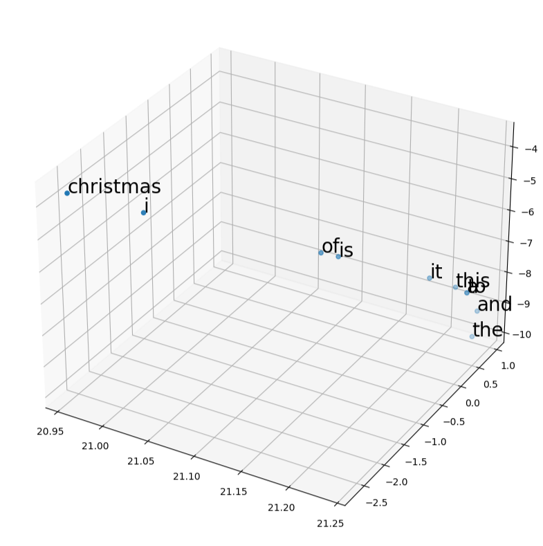
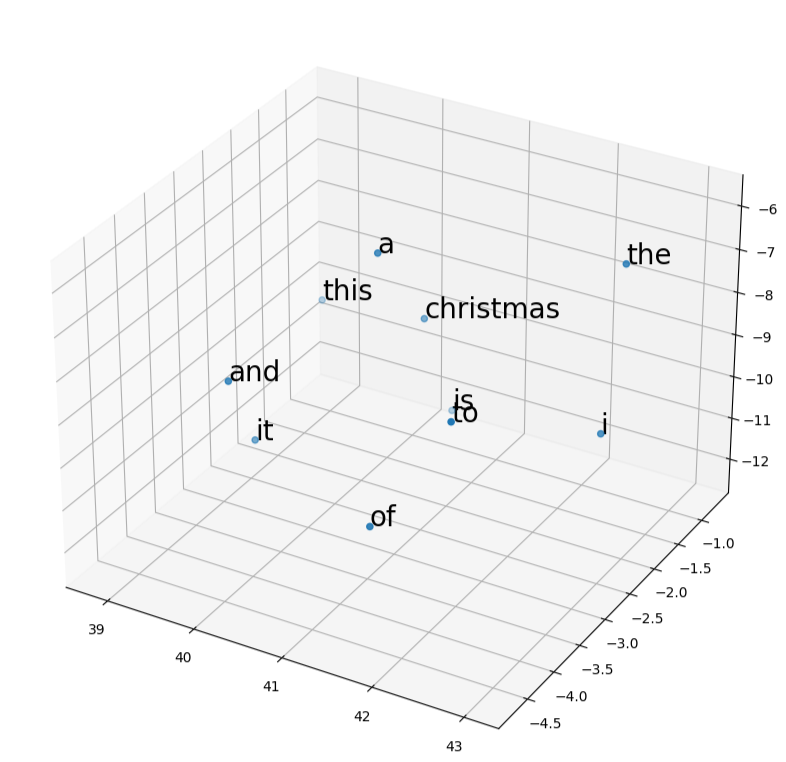
keyedvectors = KeyedVectors.load('P11_Q2_word2vec.wordvectors')
visualize_word_vectors(keyedvectors, 10) # visualize the first 10 words
The output should be a 3D scatter plot that looks like the one below:
-
Implement the
visualize_word_vectorsfunction and test it with the provided test cases. -
Visualize the FastText word vectors using TSNE.
-
Visualize the Word2Vec word vectors using TSNE.
-
Which model do you think works better for capturing word relationships? Why? (hint: look at the clusters of words in the plots)
-
In the FastText plot, what words are similar to each other? What words are dissimilar to each other? (hint: look at the clusters of words in the plots)
Question 5 (2 points)
Now that we know how to visualize word vectors in ways that we can easily understand, let’s look at some algorithms that computers use to compare them. Cosine similarity is a very common, simple, and powerful way to compare word vectors. It is a measure of the similarity between two vectors, and is simply the cosine of the angle between them. Obviously, there is no distinct angle between two vectors in a higher dimensional space, but we can use the linear algebraic definition of cosine similarity to calculate the angle between two vectors. The formula for cosine similarity is:
cos(theta) = (A . B) / (||A|| * ||B||)Where A and B are the two vectors, . is the dot product, and ||A|| and ||B|| are the magnitudes of the vectors. The cosine similarity will be between -1 and 1, where 1 means the vectors are identical, -1 means they are opposite, and 0 means they are orthogonal (not similar at all).
Please create a function called cosine_similarity that takes in a KeyedVectors object and two words, and returns the cosine similarity between the two words. Use numpy for the dot product (numpy.dot) and magnitudes (numpy.linalg.norm). If a word is not present, return a similarity of None. You can use the following code as a starting point:
import numpy as np
def cosine_similarity(word_vectors, word1, word2):
    # If a word is not present, return None
    # your code here

    # get the word vectors
    # your code here

    # calculate the dot product
    # your code here

    # calculate the magnitudes
    # your code here

    # return the cosine similarity
# your code here|
Cosine similarity is not just used for word vectors. It can be applied to anything that can be represented as a vector, which is anything! For example, it is often used in recommendation systems to compare how similar items are, which can be seen in places like Amazon. It can also be used in image processing to compare the similarity between images, their key points, etc. In fact, in my own research, I use cosine similarity to compare atomic structures in molecular dynamics modeling. It is a very powerful and versatile tool that can be used in many different fields. |
You can test your function using the following code:
keyedvectors = KeyedVectors.load('P11_Q3_fasttext.wordvectors')
print(cosine_similarity(keyedvectors, 'cd', 'music'))
print(cosine_similarity(keyedvectors, 'cd', 'christmas'))
print(cosine_similarity(keyedvectors, 'a', 'christmas'))
print(cosine_similarity(keyedvectors, 'a', 'is'))
print(cosine_similarity(keyedvectors, 'a', 'dog'))
print(cosine_similarity(keyedvectors, 'july', 'christmas'))
print(cosine_similarity(keyedvectors, 'the', 'impressive'))

# should output:
'''
0.9998109
0.9998211
0.9999449
0.9999108
0.99883497
0.9999105
0.9999365
'''
You should notice that all of your similarity values are quite similar to one. This is simply because we need more data! Recall the petabytes of data that models like GPT are trained on. Please pick 3 larger amounts of data to test and see how they perform. For example, you could do 5 thousand, 20 thousand, and 30 thousand. You can use the below code to help with that:
n = 3000 # how many lines to read.
wv = generate_word_vectors(read_lines('/anvil/projects/tdm/data/amazon/music.txt', n, 0), f'P11_Q5_fasttext_{n}')
keyedvectors = KeyedVectors.load(f'P11_Q5_fasttext_{n}.wordvectors')
print(cosine_similarity(keyedvectors, 'cd', 'music'))
print(cosine_similarity(keyedvectors, 'cd', 'christmas'))
print(cosine_similarity(keyedvectors, 'a', 'christmas'))
print(cosine_similarity(keyedvectors, 'a', 'is'))
print(cosine_similarity(keyedvectors, 'a', 'dog'))
print(cosine_similarity(keyedvectors, 'july', 'christmas'))
print(cosine_similarity(keyedvectors, 'the', 'impressive'))|
These will take longer to run, but it should still be less than a minute or so. If it is taking an excessive amount of time, please reach out to a TA to see if something is wrong with your code. |
Please state what values you tried, and how these values affected your cosine similarity metrics.
-
Implement the
cosine_similarityfunction and test it with the provided test cases. -
Passes tests for question 3 fasttext wordvectors
-
Test the function with 3 different amounts of lines read
-
State what values you tried, and how these values affected your cosine similarity metrics.
Question 6 (2 points)
Something that may be useful to intuitively check how well our word embeddings are is to create a similarity matrix. A similarity matrix is a matrix that shows the similarity between all pairs of words in a list. An example of what this would look like is below (in dictionary form, which is recommended):
similarity_matrix = {
    'cat': {'cat': 1.0, 'dog': 0.5, 'fish': 0.2, 'bird': 0.3},
    'dog': {'cat': 0.5, 'dog': 1.0, 'fish': 0.1, 'bird': 0.4},
    'fish': {'cat': 0.2, 'dog': 0.1, 'fish': 1.0, 'bird': 0.6},
    'bird': {'cat': 0.3, 'dog': 0.4, 'fish': 0.6, 'bird': 1.0}
}
Firstly, this allows us to more efficiently check the similarity between two words, as we don’t need to call the cosine_similarity function each time. We can simply index the dictionary. Additionally, it let’s us find interesting metrics about each word. For example, what is the most similar word to cat, or what is the most opposite word than cat.
Please create a function called similarity_matrix that takes in a KeyedVectors object, and returns a dictionary of the similarity matrix. You can use the cosine_similarity function to calculate the similarity between each pair of words. You can use the following code as a starting point:
def similarity_matrix(word_vectors, n_words=1000):
    # Create a dictionary to store the similarity matrix
    # your code here

    # Get the words from the KeyedVectors object\
    # your code here

    # Calculate the cosine similarity between each pair of words
    # your code here

    # Return the similarity matrix
    # your code here
You can check that your function works by using the following code:
n = 25000 # how many lines to read.
wv = generate_word_vectors(read_lines('/anvil/projects/tdm/data/amazon/music.txt', n, 0), f'P11_Q5_fasttext_{n}')
keyedvectors = KeyedVectors.load(f'P11_Q5_fasttext_{n}.wordvectors')

similarity_matrix_25k = similarity_matrix(keyedvectors)

print(similarity_matrix_25k.get('cd', {}).get('music',None))
print(similarity_matrix_25k.get('cd', {}).get('christmas',None))
print(similarity_matrix_25k.get('a', {}).get('christmas',None))
print(similarity_matrix_25k.get('a', {}).get('is',None))
print(similarity_matrix_25k.get('a', {}).get('dog',None))
print(similarity_matrix_25k.get('the', {}).get('the',None))

# should output:
'''
0.31273866
0.3474876
0.33200315
0.18050662
None
1.0
'''|
While I would have liked you to create a similarity matrix for all words, this will take a very very long amount of time. The P11_Q5_fasttext_25000.wordvectors has 53000 words, and from my testing it will take ~5.5 hours to generate the similarity matrix between all of them, depending on your implementation. Feel free to do this if you want, but it is not necessary to complete the project |
Additionally, let’s sort the similarity dictionaries for cd, music, and christmas, to see which words are most and least similar to them.
An example of this is shown below, showing the 5 most and least similar words to 'the'
similarities_the = similarity_matrix_25k.get('the', {})
similarities_the_sorted = sorted(similarities_the.items(), key=lambda x: x[1], reverse=True)
print(similarities_the_sorted[:6]) # 5 most similar words to 'the'
print(similarities_the_sorted[-6:]) # 5 least similar words to 'the'
Please do the same for cd, music, and christmas. Does your similarity matrix make sense? What does this tell you about how accurate your word embeddings are?
-
Implement the
similarity_matrixfunction and test it with the provided test cases. -
Passes test cases for 25000 lines read
-
Get the 5 most and least similar words to
cd,music, andchristmas. -
Does your similarity matrix make sense? What do the most similar and least similar words tell you about the accuracy of these word embeddings?
Submitting your Work
Once you have completed the questions, save your Jupyter notebook. You can then download the notebook and submit it to Gradescope.
-
firstname_lastname_project11.ipynb
|
You must double check your You will not receive full credit if your |