TDM 30200: Project 08 - Feature Selection (Regularization)
Project Objectives
This project aims to provide students with an understanding of feature selection techniques through the application of regularization methods, specifically Ridge Regression, and LASSO. By utilizing these methods on the Lahman Baseball Database in R, students will explore how selecting relevant variables can improve model performance, reduce overfitting, and enhance interpretability.
|
For this project, we will use R instead of Python, as it offers a more streamlined and efficient approach to modeling. In this project, rather than focusing on which programming language is used, we will emphasize why certain tools and techniques are applied. For ease of understanding, we will demonstrate the concept using a simple linear model. However, the regularization methods we cover here are based on the same principles used in many machine learning algorithms and neural network models, too. Please use the |
Dataset
We will work with the Lahman Baseball Database, which is available in R through the Lahman package.
Introduction
One of the fundamental steps in modeling is identifying the relevant variables. While machine learning models can handle large datasets and a high number of features, strong dependencies among variables can reduce the reliability of model parameters. Also, when the number of variables (p) exceeds the number of observations (n), the difficulties become more significant.
For instance, in linear models, having p > n means that the system of equations is underdetermined, leading to infinitely many possible solutions. This can cause instability in parameter estimation and increase the risk of overfitting. To address this issue, regularization techniques such as Ridge regression or LASSO, can be used to impose constraints on the model and improve generalization.
Questions
Question 1 (2 points)
We’ve previously utilized the Batting table from the Lahman dataset, which contains batting statistics. Specifically, we examined the relationship between Homeruns (HR) and Runs Batted In (RBI), noting how HR influences RBI. However, the Batting table offers numerous other variables that can enhance our models. To explore these variables, execute the following R code first:
library(Lahman)

names(Batting)
To gain detailed information about the variables in the Batting table, use the ?Batting command in R to access the documentation.
People is another table including player names, date of births and demographics for baseball players. It provides more details about players and it shares unique 'playerID' which can be used to merge Batting and People data sets. People contains 26 variables, but many of them are expected to have a large number of missing (NA) values. For instance, since the data includes records up to 2023, the death- columns will have many empty entries, as most players in recent years are alive. Additionally, these variables are not meaningfully related to RBI, so they do not need to be considered in the modeling process.
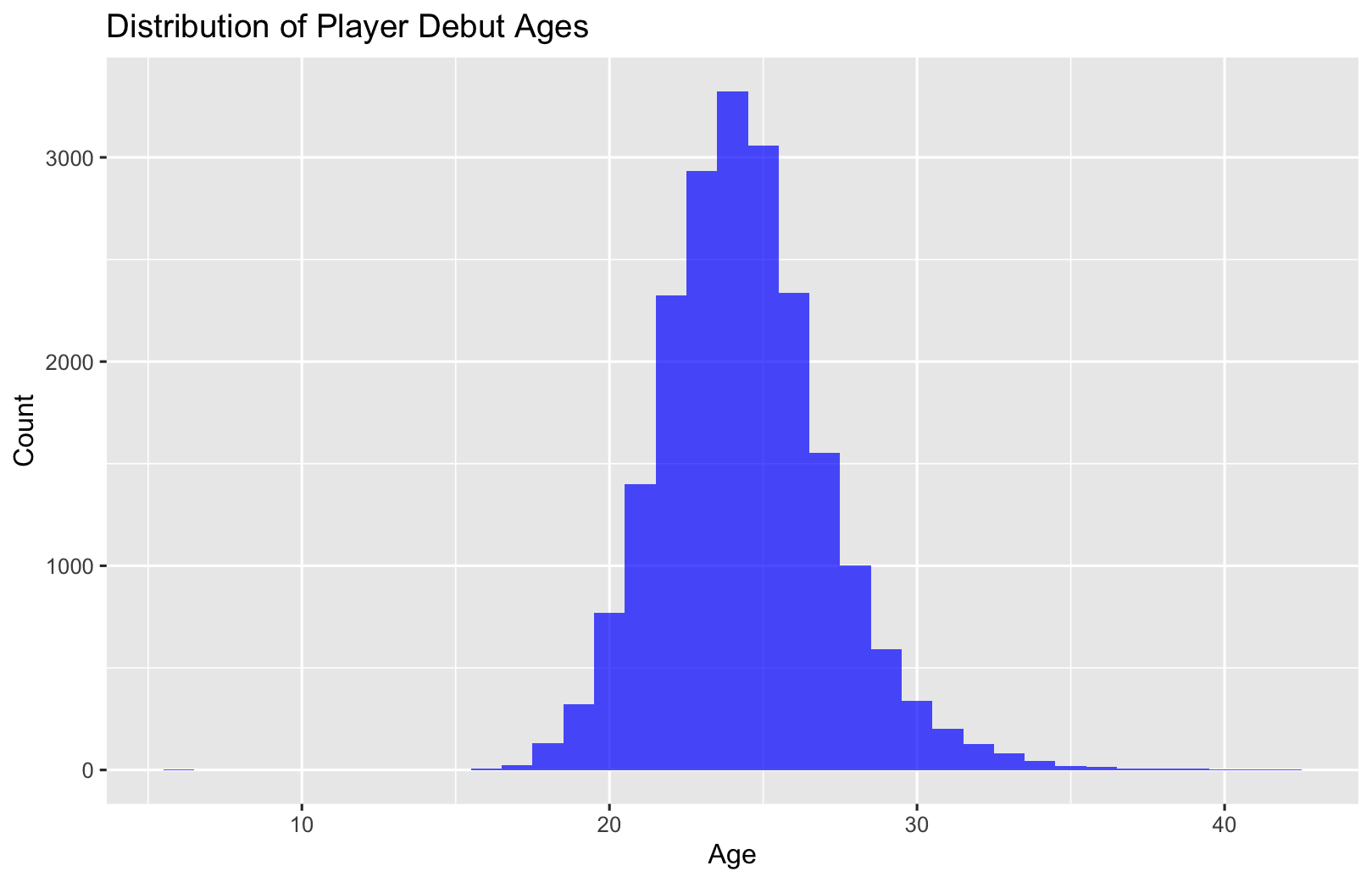
Some variables may provide interesting insights about the data but be less important for modeling. For example, while the age at which players make their debut can be an intriguing variable, their actual age might contribute more significantly to the model. Additionally, the most common birthplaces highlight Major League Baseball’s international reach, but its contribution to the model may be less. For curious readers, below are chart and tables related to debut ages and the most common (first ten) birthplaces. (Reproducing the visual and table is not required for the project.)
Most common birth countries
| Birth country | n |
|---|---|
USA |
18098 |
Dominican Republic |
890 |
Venezuela |
472 |
Puerto Rico |
281 |
Canada |
266 |
Cuba |
237 |
Mexico |
147 |
Japan |
76 |
Panama |
70 |
Ireland |
50 |
|
R code for Debut Age: |
The extensive variables within the Batting and People tables offer numerous opportunities for model development. Building upon our previous linear modeling approach, we aim to explain the variation in our target variable, Runs Batted In (RBI), using a broader set of predictors. To achieve this, we will first merge the datasets using the unique identifier, playerID:
# Merge two datasets
full_data <- Batting %>%
  left_join(People, by = "playerID") %>%
  na.omit()
The People dataset contains players' birth years, a potentially valuable predictor. However, given the dataset’s wide historical range (1871-2023), directly including birth year might not be optimal. Instead, calculating players' ages and incorporating that variable would better account for age-related differences in performance.
-
1.1. Check out column names, display the first six lines and examine summary statistics for
BattingandPeopledatasets. -
1.2. Merge
BattingandPeopledatasets by playerID as the join key. -
1.3. Calculate the age of each player (based on birthYear and yearID) and add it as a new column named 'age' to the merged dataset.
|
For the ease of reading, all variables are added with their codes and explanations in Appendix at the end of this document. Tables includes all variables for |
Question 2 (2 points)
Prior to modeling, let’s examine a heatmap of the numeric variables intended for use in our model.
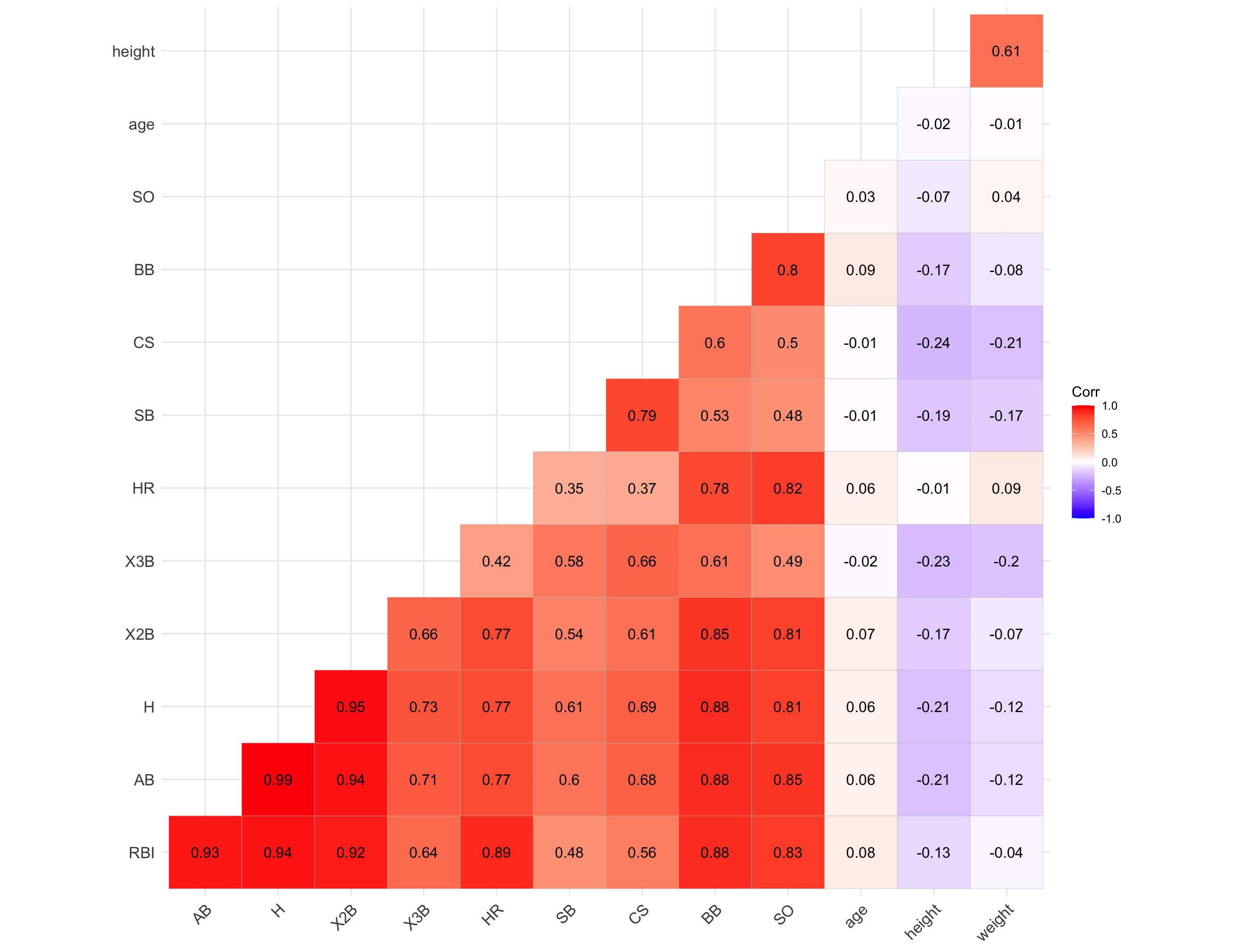
Data visualization offers essential clues to understanding your data before initiating the modeling process. For instance: At Bats (AB), Hits (H), and Doubles (X2B) are highly correlated because they follow a natural hierarchy in baseball statistics. AB represents a player’s batting opportunities, H is a subset of AB, counting successful hits, and X2B is a further subset, representing only doubles. Since more at-bats generally lead to more hits, and more hits increase the likelihood of doubles, these variables are inherently linked, resulting in strong correlations. In most cases, H (Hits) may be the best choice because it captures a player’s ability to reach base successfully, encompassing both singles and extra-base hits while avoiding redundancy.

The source of the picture is apnews accessed at 03/08/2025.
The following linear model uses as much variables as possible to explain the changes in target, RBI variable (The age variable was generated in Question 1.3).
# Fit a linear model
lm_model <- lm(RBI ~ yearID + lgID + H + X3B + HR + SB + CS + BB + SO + age + height + weight + bats, data = full_data)

# Display model summary
summary(lm_model)
Although a linear model provides P-values as evidence for variable selection, shrinkage or regularization (e.g., LASSO, Ridge) methods are used for variable selection because P-values can sometimes be misleading, especially when the sample size is large, or when variables are highly correlated with one another. In such cases, a variable with a high P-value might still be relevant for the model, but its contribution isn’t significant enough to pass the threshold. In some cases, especially when dealing with a large number of variables, instead of focusing on interpreting the output, you may want the model to perform both parameter estimation and variable selection simultaneously. Furthermore, many machine learning algorithms, due to their lack of interpretability, do not provide evidence (such as P-values) of which variables contribute to the model.
Variable selection (feature engineering) in statistical models is crucial for improving both the model’s performance and interpretability. By choosing only the most relevant variables, we can simplify the model, making it easier to understand and interpret, which is particularly important in fields where the relationships between variables are essential. Additionally, variable selection helps prevent overfitting, a common issue when too many irrelevant variables are included, which can lead to a model that fits the noise in the data rather than the underlying patterns. A more focused model with fewer predictors tends to generalize better to new data, leading to improved prediction accuracy. By selecting the right variables, we can also reduce computational costs, as fewer predictors mean less memory and processing power are required, which is especially important in large datasets.
While shrinkage methods continue to evolve and new ones (such as Elastic net) are introduced, understanding Ridge and LASSO provides a strong foundation for grasping more advanced techniques. Now, let’s recall the linear model we discussed earlier and review its mathematical representation with a single predictor.
$RBI_{i} = \beta_0 + \beta_1 HR_{i} + \epsilon_{i}$,
where:
-
$\beta_0 =$ Common starting point for all players (overall intercept)
-
$\beta_1 =$ Average effect of HR across all players (overall slope)
-
$\epsilon_{i} =$ Error term (noise comes from modeling)
We can replace the variable names in the model with their symbolic representations:
$y_{i} = \beta_0 + \beta_1 x_{i} + \epsilon_{i}$.
Generalize it for $p$ variables:
$y_{ij} = \beta_0 + \sum_{j = 1}^{p}\beta_j x_{ij} + \epsilon_{ij}$.
Since we are looking for the best estimates for the unknown $\beta$ parameters in this model, we want to minimize $\epsilon_{ij}$ as much as possible. The method that provides the best estimates for these parameters is the least squares approach, which finds $\beta$ values that minimize the residual sum of squares (RSS):
$RSS = \sum_{i = 1}^{n}(y_i - \beta_0 - \sum_{j = 1}^{p}\beta_j x_{ij})^2$.
Even without prior knowledge of this method, if we were to consider the best way to predict $y_i$ based on the given model, our natural goal would be to make both sides of the equation as close as possible. The variables in the model are known, and the parameters are estimated from the data, while $\epsilon$ represents an uncontrollable term arising from inherent uncertainty. Since this term cannot be eliminated, our objective is to minimize its impact. Rather than minimizing $\epsilon$ directly, we minimize its squared value to ensure that positive and negative errors do not cancel each other out.
-
2.1. Fit a linear model with RBI as the dependent (target) variable, including all the independent variables you want to incorporate from both tables. You may use the same variables included in the full model from the previous question.
-
2.2. What is model interpretability?
-
2.3. Consider a linear model where RBI is the target (dependent) variable, and HR and age are the independent variables. We can fit this model using the
lmfunction and extract the model parameters with the following R command:
lmmodel <- lm(RBI ~ HR + age, data = full_data)

coef(lmmodel)
Using the estimated coefficients from this model, calculate the Residual Sum of Squares (RSS) manually. Instead of using built-in residual functions in R, compute RSS by directly applying the following formula:
$RSS = \sum_{i = 1}^{n}(y_i - \beta_0 - \sum_{j = 1}^{p}\beta_j x_{ij})^2$
Question 3 (2 points)
Shrinkage/regularization methods introduce penalties when minimizing the Residual Sum of Squares (RSS), also known as the least squares loss function or objective function. These methods incorporate a penalty term into the RSS minimization process when estimating parameter values. Adjusting the magnitude of this penalty term influences the estimated parameters, helping to control model complexity and prevent overfitting.
Imagine you’re packing a suitcase for a trip. You want to bring everything you might need, but if you pack too much, your suitcase becomes heavy and difficult to carry. Shrinkage methods like Ridge and LASSO work similarly in a statistical model. Without any penalty, the model can include as many variables as possible, making it complex and potentially overfitting the data. However, by adding a penalty term (like an airline imposing a weight limit on luggage), the model is forced to prioritize important variables while reducing the impact of less significant ones. Ridge regression acts like a soft weight limit—allowing you to bring all your items but compressing them slightly to make the suitcase more manageable. LASSO, on the other hand, is stricter, forcing you to completely remove unnecessary items to meet the weight limit. This way, shrinkage methods prevent your model from becoming too complex while ensuring it still performs well.
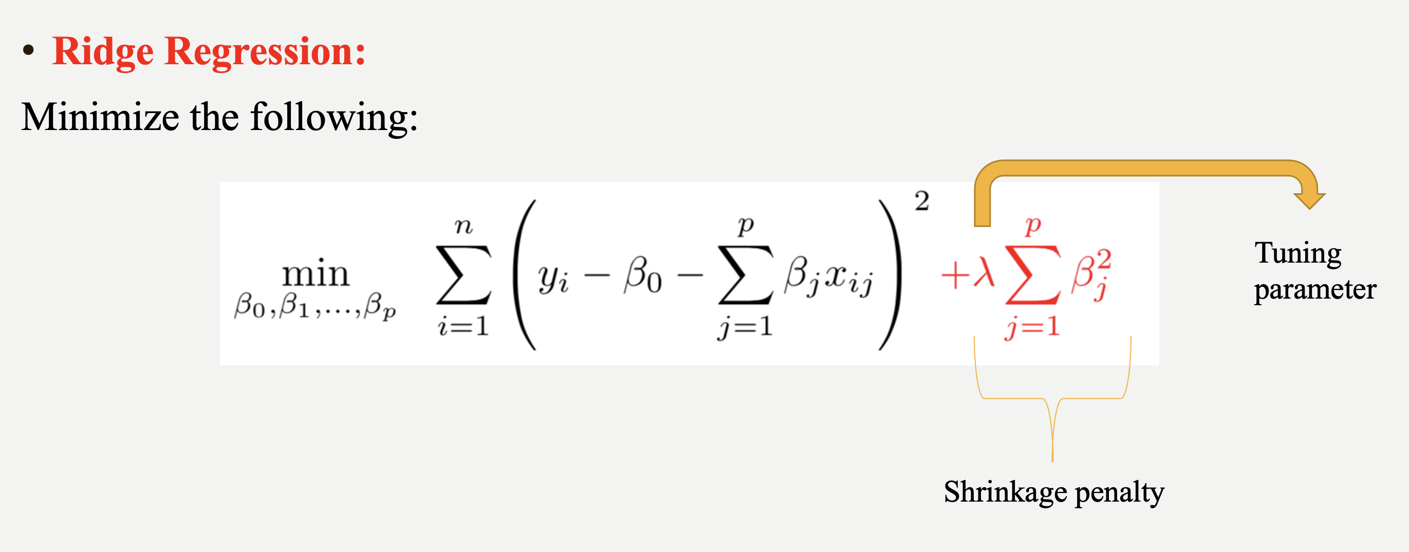
Ridge regression adds a penalty term to the least squares objective function. This penalty term (L-2 penalty) is proportional to the squared magnitude of the coefficients, shrinking them towards zero:
$\sum_{i = 1}^{n}(y_i - \beta_0 - \sum_{j = 1}^{p}\beta_j x_{ij})^2 + \lambda \sum_{j = 1}^{p} \beta_j^2$
where $\lambda$ is a hyperparameter or it is called as tuning parameter.
Before moving on to the next paragraph, I recommend taking a minute to pause and consider what a hyperparameter is, how it differs from a parameter, and how it can be found in a general model setting.
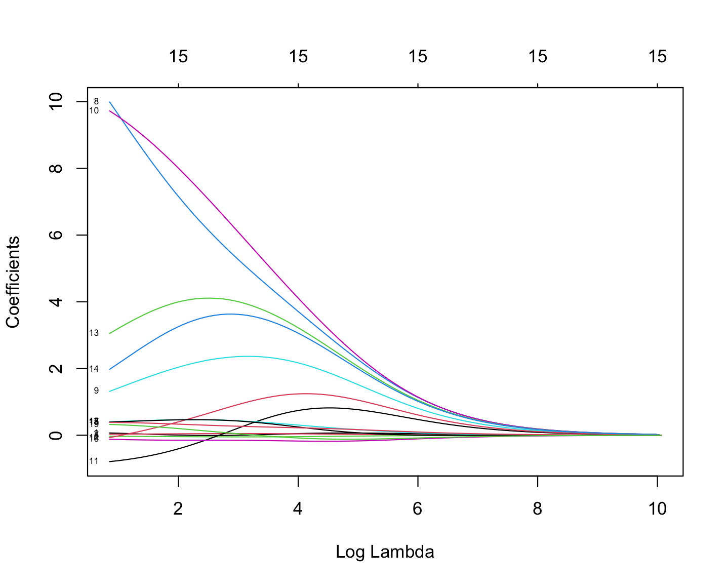
As illustrated in the figure above, we can control the magnitude of the $\beta$ coefficients by adjusting the value of the tuning parameter, $\lambda$. During the minimization process, the Residual Sum of Squares (RSS) is minimized while simultaneously penalizing the size of the coefficients. This leads to the following relationships:
-
If $\lambda \rightarrow 0$, the estimated parameter values converge to those obtained from ordinary least squares.
-
If $\lambda \rightarrow \infty$, the ridge regression coefficients shrink toward zero.
|
Before using shrinkage methods like Ridge or LASSO, it is crucial to scale the predictor variables. These methods apply a penalty to the regression coefficients, and since the penalty depends on the magnitude of the coefficients, variables with larger scales can dominate the shrinkage process. For example, if one variable is measured in thousands (e.g., salary in dollars) and another in single digits (e.g., years of experience), the penalty term will affect the variable with larger numerical values, even if both have similar importance in predicting the outcome. This can lead to biased coefficient estimates and misinterpretation of variable importance. To avoid this issue, standardization (subtracting the mean and dividing by the standard deviation) ensures that all variables contribute equally to the shrinkage process. |
The programming languages such as R and Python estimates the parameter for different values of $\lambda$. glmnet is one of the libraries in R which can be used to run a regularization method. glmnet function can run several types of regression models with a grid of values for the regularization parameter, $\lambda$. Here is the example code:
# Load necessary library
library(glmnet)

# Prepare the matrix of predictors (excluding the response variable)
X <- model.matrix(RBI ~ yearID + lgID + H + X3B + HR + SB + CS + BB + SO + age + height + weight + bats, data = full_data)[, -1]
y <- full_data$RBI

# Standardize predictors
X_scaled <- scale(X)

# Replace NaNs (from zero variance) with 0
X_scaled[is.na(X_scaled)] <- 0  # lgID variable has some non-observed values in the data

# Fit ridge regression model (alpha = 0 for ridge)
ridge_model <- glmnet(X_scaled, y, alpha = 0)
coef(ridge_model)
ridge_model$lambda
The plot below illustrates how coefficient values vary with changes in log-lambda in Ridge regression.
-
3.1. What is the role of $\lambda$ in penalized RSS?
-
3.2. Perform Ridge regression using the same variables from Question 2.1.
-
3.3. How many different $\lambda$ values were tested in the Ridge regression in 3.2?
Question 4 (2 points)
While Ridge Regression effectively shrinks coefficients towards zero, it rarely eliminates them entirely. This means that even with Ridge, you might end up with a model containing many features, some of which may be redundant. To address this, we can use LASSO (Least Absolute Shrinkage and Selection Operator). LASSO, like Ridge, uses a penalty term to regularize the model, but it employs the L1 norm (absolute value) instead of the L2 norm (square). This crucial difference allows LASSO to perform feature selection by driving some coefficients to exactly zero, effectively removing those features from the model. This time, the penalized RSS looks as follows:
$\sum_{i = 1}^{n}(y_i - \beta_0 - \sum_{j = 1}^{p}\beta_j x_{ij})^2 + \lambda \sum_{j = 1}^{p} |\beta_j|$
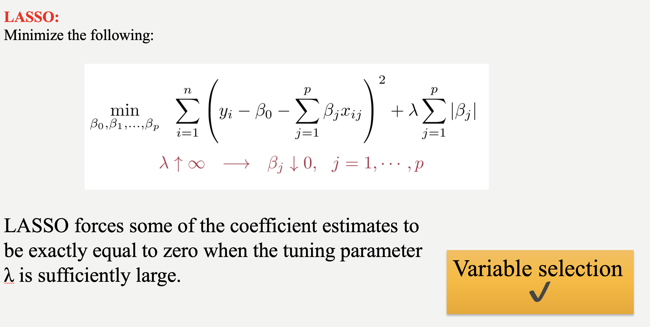
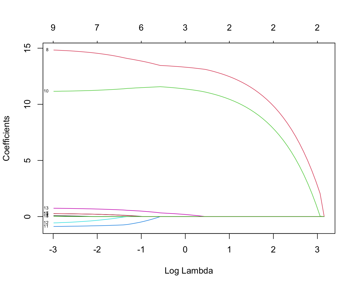
Similar to ridge, we have a tuning parameter, $\lambda$ and changing its value changes the magnitude of parameter coefficients. R code is also exactly the same as the ridge regression, the only difference is that using alpha = 1 instead of 0 in the glmnet function.
The following plot shows how coefficient values are changing with the change in Log Lambda in LASSO regression.
-
4.1. Perform LASSO regression using the same linear model and variables from Question 2.1.
-
4.2. How many different $\lambda$ values were tested in the LASSO regression in 4.1?
Question 5 (2 points)
Up to this point, we have run models but have not yet determined the optimized model or final parameter estimates. Why is that?

So far, we have not performed any feature selection; we have only applied regularization methods across different $\lambda$ values and reported the results. To identify the final model, we must use cross-validation to evaluate each $\lambda$ on unseen test data. The optimal $\lambda$ is then selected based on model performance. Only after this step can we determine which explanatory variables contribute most effectively to explaining the variation in the dependent variable.
With the coding and cross-validation knowledge we’ve gained so far, we have the tools to implement cross-validation for regularization in our models. However, R provides the cv.glmnet function, which streamlines this process with a concise set of code. If you feel confident in your understanding of shrinkage/regularization and cross-validation, you can use this function to perform feature selection. But if you think you need more practice with these concepts, I recommend implementing cross-validation manually before using cv.glmnet.
Let’s proceed with feature selection with cross-validation for LASSO:
# Perform LASSO regression using cross-validation
set.seed(42) # optional, just for reproducibility
lasso_cv <- cv.glmnet(X, y, alpha = 1)  # alpha = 1 for LASSO

# Extract the best lambda value
best_lambda <- lasso_cv$lambda.min
print(paste("Best Lambda:", best_lambda))-
5.1. Fit Ridge and LASSO regression models using their respective cross-validated optimal lambda values.
-
5.2. Extract and display the coefficients selected by the final LASSO and Ridge model.
|
Below is a general representation of shrinkage methods, which can inspire you to create your own regularization approaches. 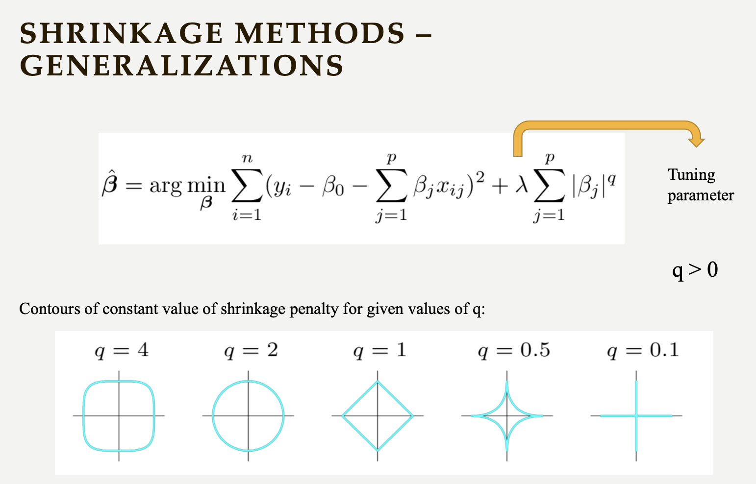
|
Appendix 1
Batting Data Variables
| Variable Code | Explanation |
|---|---|
playerID |
Player ID code (links to People dataset) |
yearID |
Year |
stint |
Player’s stint (order of appearances within a season) |
teamID |
Team; a factor |
lgID |
League; a factor with levels AA, AL, FL, NL, PL, UA |
G |
Games: number of games in which a player played |
AB |
At Bats |
R |
Runs |
H |
Hits: times reached base because of a batted, fair ball without error by the defense |
X2B |
Doubles: hits on which the batter reached second base safely |
X3B |
Triples: hits on which the batter reached third base safely |
HR |
Homeruns |
RBI |
Runs Batted In |
SB |
Stolen Bases |
CS |
Caught Stealing |
BB |
Base on Balls |
SO |
Strikeouts |
IBB |
Intentional walks |
HBP |
Hit by pitch |
SH |
Sacrifice hits |
SF |
Sacrifice flies |
GIDP |
Grounded into double plays |
People Data Variables
| Variable Code | Explanation |
|---|---|
playerID |
A unique code assigned to each player. Links to other files. |
birthYear |
Year player was born |
birthMonth |
Month player was born |
birthDay |
Day player was born |
birthCountry |
Country where player was born |
birthState |
State where player was born |
birthCity |
City where player was born |
deathYear |
Year player died |
deathMonth |
Month player died |
deathDay |
Day player died |
deathCountry |
Country where player died |
deathState |
State where player died |
deathCity |
City where player died |
nameFirst |
Player’s first name |
nameLast |
Player’s last name |
nameGiven |
Player’s given name (typically first and middle) |
weight |
Player’s weight in pounds |
height |
Player’s height in inches |
bats |
Player’s batting hand (left (L), right ®, or both (B)) |
throws |
Player’s throwing hand (left (L) or right ®) |
debut |
Date that player made first major league appearance |
finalGame |
Date that player made first major league appearance (blank if still active) |
retroID |
ID used by Retrosheet, www.retrosheet.org/ |
bbrefID |
ID used by Baseball Reference website, www.baseball-reference.com/ |
birthDate |
Player’s birthdate, in as.Date format |
deathDate |
Player’s deathdate, in as.Date format |
Appendix 2
R Code for Correlation Hep Map
library(ggcorrplot)

# Merge Batting and People tables - numeric variables
corrdata <- Batting %>%
  left_join(People, by = "playerID") %>%
  mutate(age = yearID - birthYear) %>%
  select(RBI, yearID, AB, H, X2B, X3B, HR, SB, CS, BB, SO, age, height, weight) %>%
  na.omit()  # Remove rows with NA values

# Compute correlation matrix
cor_matrix <- cor(corrdata, use = "pairwise.complete.obs")

# Plot correlation heatmap
ggcorrplot(cor_matrix, lab = TRUE, type = "lower", colors = c("blue", "white", "red"))
Submitting your Work
Once you have completed the questions, save your Jupyter notebook. You can then download the notebook and submit it to Gradescope.
-
firstname_lastname_project1.ipynb
|
You must double check your You will not receive full credit if your |