TDM 10200: Project 6 - Manipulating Data
Project Objectives
Motivation: Often data is messy or too big to work with. Knowing how to create subsets and clean up data values is a valuable skill.
Context: We will use a few different datasets to practice data manipulation.
Scope: Python, data cleaning, subsets, bins
Make sure to read about, and use the template found on the template page, and the important information about project submissions on the submission page.
Dataset
-
/anvil/projects/tdm/data/flights/subset/2006.csv
-
/anvil/projects/tdm/data/icecream/combined/products.csv
-
/anvil/projects/tdm/data/flights/subset/1997.csv
|
If AI is used in any cases, such as for debugging, research, etc., we now require that you submit a link to the entire chat history. For example, if you used ChatGPT, there is an “Share” option in the conversation sidebar. Click on “Create Link” and please add the shareable link as a part of your citation. The project template in the Examples Book now has a “Link to AI Chat History” section; please have this included in all your projects. If you did not use any AI tools, you may write “None”. We allow using AI for learning purposes; however, all submitted materials (code, comments, and explanations) must all be your own work and in your own words. No content or ideas should be directly applied or copy pasted to your projects. Please refer to GenAI page in the example book. Failing to follow these guidelines is considered as academic dishonesty. |
Flights
The flights dataset is huge, with files from 1987 to 2023, each with respective subset datasets just to make the data reasonable to work with. The flights data provides numerous opportunities for data exploration with 7,141,922 rows of data from 2006 and 5,411,843 rows from 1997 alone. These subsets contain information about when each flight took place, as well as different factors like how long they took, specifics like flight numbers, and more. There are, of course, empty or messy values, but there is so much data that this does not make too much of an impact for what we will be doing.
There are 29 columns and millions of rows of data. Some of these columns include:
-
Month: numeric month values -
DayofMonth: day of month (1 - (28 up to 31)) -
DayOfWeek: numeric day values -
DepTime: flight departure time in military time shorthand -
ArrTime: flight arrival time in military time shorthand -
AirTime: flight time, in minutes -
Origin: abbreviation values for origin airport -
Dest: abbreviation values for destination airport
Ice Cream Products
The Ice Cream dataset is on the smaller side, containing just a few hundred rows of data. This dataset contains information about four different ice cream brands' products, with product information that would make purchasing easier, such as the description, how the product was rated, and what ingredients it contains.
Some of the columns (description, ingredients) of this dataset are not particularly useful given our current skillset, and can make looking at rows of this data not so easy. Which makes taking specific columns (like the rating column) and isolating them for work ideal.
The rating column is each ice cream’s customer rating on a scale of 0 - 5.
Questions

|
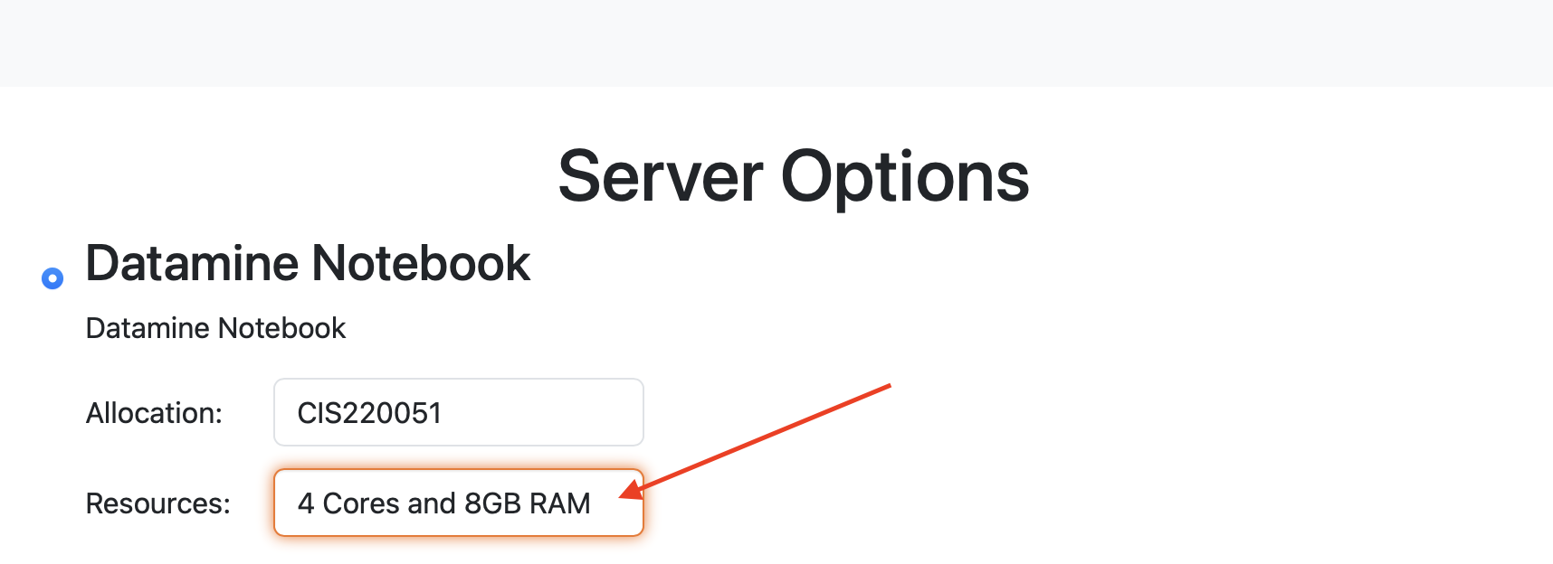
You will need to use 4 cores for this project. |
Question 1 (2 points)
The flights dataset is much too large to work with all at once, so we are going to be working with the 2006 subset. This dataset contains all of the same columns as the other flights datasets, just only for the flights for which the year was 2006.
Use the pandas library to read in the 2006 flights subset data as myDF.
You will notice a star (see below) at the beginning of the code line for this dataset, as it takes some time to load in Anvil due to its large size:

If some of the columns do not show up (they shown as … in the output) when looking at the .head() of the dataset, use pd.set_option('display.max_columns', None) to set a high maximum number of columns that can be displayed at a time.
Create pa_flights containing only the flights that have a destination of the Philadelphia International Airport (PHL).
Remember, when subsetting a dataframe in Python, we can select to keep only the data which matches a certain condition:
# Select the rows where Food equals "pizza"
pizza = MyHungryData[MyHungryData['Food'] == "pizza"]
Using this same approach, you can filter flights with destination "PHL".
If you look at the shape of this pa_flights, you will see that this subset still contains many rows of data. PHL is a very popular airport, with many flights leaving from and arriving there. Show how many unique Origin spots there are for flights going to PHL.
|
Use |
Using the flights' origins, use .groupby() to find the average AirTime for each flight in the pa_flights data. The standard way of doing this is df.groupby("col1")["col2"].mean(). This output will show the average air time for each unique flight origin, with a destination of PHL.
To sort these results from highest to lowest average, set ascending to equal False in .sort_values().
Make a second temporary dataframe containing the data for flights ending at PHX (Dest column). Then use .groupby() to find the average AirTime across each flight origin, and sort to find the top results.
1.1 How many flight origins did PHL have in 2006?
1.2 What was the average AirTime for flights leaving SFO in pa_flights in 2006?
1.3 What was the average AirTime for flights leaving HNL in az_flights in 2006?
Question 2 (2 points)
In Question 1, we only used the destination of two selected airports. Here, use the top 20 destinations when comparing each average air time of each origin-and-destination pair.
The function .value_counts() will return the names and values of a search. These results default to sorting by highest to lowest value. Take the top 20 most popular destination airports and make a new variable top_20.
Use .head(20) to take the first 20 results of an output.
|
|
We have already used .isin() just a bit in Project 4: it checks whether or not a value is included in another set of values. In this example, we can use .isin() to filter myDF so that we only keep the rows where the destination (Dest) is one of the values inside the list top_20.
This will give you a new dataframe, containing only the flights going to any of those top 20 destinations:
top_dests_df = myDF[myDF["Dest"].isin(top_20)]In the .groupby() method, we are also able to work with multiple column pairs. For example, we can show the average AirTime across each Origin and Dest pair for the top 20 destination pairs as follows:
result = top_dests_df.groupby(["Origin", "Dest"])["AirTime"].mean()A nice way to view result is to run result.unstack(). This formats results as a dataframe rather than a series, with
-
Rows = Origin,
-
Columns = Dest,
-
Cells = mean AirTime.
2.1 Save the 20 most popular airport destinations as top_20.
2.2 Display the airports that are in top_20.
2.3 Display the .head() of the dataframe result.
Question 3 (2 points)
For this question, read in the ice cream products file from /anvil/projects/tdm/data/icecream/combined/products.csv as ice_cream.
View the value counts of the rating column. This shows the counts of each rating (from 0 to 5), and is helpful, but there is something more we can find.
To better understand this column and how each ice cream was received, we could add labels to each range of rating.
The .cut() and .qcut() functions in Python are used for dividing continuous data into "bins". These two functions allow for you to group data points, which is useful for analyzing trends or patterns within those groups.
|
In In |
With the ice_cream dataset, use .qcut() with q=4 to classify the four rating ranges. Apply labels to define each range:
-
"Wouldn't Recommend": min - 25% -
"Needs Improvement": 25% - 50% -
"Solid Choice": 50% - 75% -
"Fan Favorite": 75% - max
|
The ranges are automatically decided by |
3.1 Use .describe() to view the statistics of the rating column.
3.2 What ranges did .qcut() create? (View before applying labels).
3.3 Display the first 5 rows of ice_cream once rating_phrases has been created.
Question 4 (2 points)
For this question, read in the 1997 flights subset dataset as my_flights. This dataset has the same structure as the 2006 flights data we used earlier, but it only includes flights from the year 1997.
|
Your kernel may die while trying to read in this dataset. This means you either rerun everything in this notebook (the kernel may die again), OR just re-import in pandas and only rerun |
In this data, the DepTime column tracks what time each flight departs. This column does not display time like we would expect, instead using a range from 1 (00:01am) to 2400 (midnight). There are a lot of different values in this column.
One way to make this data more readable is to add some set ranges using the .cut() function. Like before with the ice cream data, this would allow us to analyze the data based on a smaller number of sets rather than each individual time.
Build a .cut() function to break the DepTime column up into sections. Display the value counts of this to get each groups' number of occurrences.
|
We use Meaning:
|
|
Using the bins |
Add a corresponding label to each bin of DepTime. For an example of a full set of labels you could use: "Late Night", "Early Morning", "Morning", "Late Morning", "Afternoon", "Early Evening", "Evening", "Night".
Save the DepTime bins and their labels as the new column depart_times and print the value counts of depart_times.
Use sort=False in .value_counts() if you want to order based on the values rather than their counts.
Using the same method you used to create depart_times, break ArrTime into bins with labels, and create the column arrival_times.
4.1 Create depart_times based on the bins (and their respective labels) from DepTime.
4.2 Create arrival_time based on the bins (and their respective labels) from ArrTime.
4.3 Which departure time is the busiest? Which arrival time is the busiest?
Question 5 (2 points)
Still within the 1997 flights dataset, there are the columns Month, DayOfWeek, and AirTime. Something interesting we could find is how the day of the week and the month out of the year affect the total air time.
Use the form df[df["col"] == value] to make a saved selection of rows for a specific month. For example:
march = my_flights[my_flights["Month"] == 3]View the value counts of the DayOfWeek column for this month (march in our example). As expected, the counts of the flights for each day of this month are all within reasonable range of each other.
Do this again, just on all of the months (together) from the original dataframe.
To view the total AirTime for each DayOfWeek, use the .groupby() method. You should have 7 value categories
Using .groupby(), we are able to create a more complicated dataframe, where we choose an x-axis, a y-axis, and for what values the cells in the table are being calculated. In this case, use AirTime as the values, and show Month and DayOfWeek on the axes, as following:
my_flights.groupby(["DayOfWeek", "Month"])["AirTime"].sum().unstack()Create a second dataframe using the same example code, but calculate the mean rather than the sum.
5.1 Compare the DayOfWeek value counts from your selected month to that of all of the months put together.
5.2 Display the dataframe that shows the total airtime of flights across the days of the week and the months.
5.3 Display the dataframe that shows the average airtime of flights across the days of the week and the months.
Submitting your Work
Once you have completed the questions, save your Jupyter notebook. You can then download the notebook and submit it to Gradescope.
-
firstname_lastname_project6.ipynb
|
It is necessary to document your work, with comments about each solution. All of your work needs to be your own work, with citations to any source that you used. Please make sure that your work is your own work, and that any outside sources (people, internet pages, generative AI, etc.) are cited properly in the project template. You must double check your Please take the time to double check your work. See submission page for instructions on how to double check this. You will not receive full credit if your |