Introduction to Linear Mixed Models
Project Objectives
This is a past seminar project where we introduced linear mixed effects models and explore how they account for subject-level variability in longitudinal data. Although it was used for teaching purposes, it is still useful for introducing linear mixed models.
Dataset
-
/anvil/projects/tdm/data/sleepstudy/sleepstudy.csv
-
sleepstudy : A longitudinal reaction time dataset commonly used to demonstrate linear mixed effects models. Please refer to the sleepstudy documentation page on CRAN for more info.
Introduction to Linear Mixed Effects Models
Mixed effects models are called "mixed" because they combine fixed effects and random effects within the same model. Fixed effects describe the overall population relationship. These are the primary effects we want to estimate, similar to the coefficients in a standard linear regression. Random effects capture group-level variation by allowing certain parameters (such as intercepts or slopes) to vary across groups. They allow certain parameters (such as intercepts or slopes) to vary across groups of repeated measurements.
When we collect repeated measurements from the same individual, those observations are not independent. A mixed model accounts for this dependency by allowing each individual to deviate from the overall population trend.
Consider our sleep study dataset:
-
X: Days of sleep deprivation,
-
Y: Reaction time,
-
Each subject represents a different individual.
If we fit a simple linear regression:
$Reaction \sim \beta_0 + \beta_1 \cdot Days$.
In this model, we assume:
-
All subjects share the same baseline reaction time,
-
Reaction time increases at the same rate for everyone,
-
Any remaining differences are random noise.
However, when we examine the data more closely:
-
Some individuals begin with faster reaction times (lower intercepts),
-
Others begin with slower reaction times (higher intercepts),
-
The overall trend may be similar, but subjects differ in their starting point.
What a Mixed Model Does
Rather than forcing one line to describe everyone, a mixed model assumes that there is an overall population trend, and individuals vary around that trend. Instead of writing $Reaction \sim Days$, we specify:
$Reaction \sim Days + (1 \mid Subject)$
This notation means:
-
$Days$ represents the fixed effect (the average slope across all subjects),
-
$(1 \mid Subject)$ allows each subject to have their own intercept.
As a result:
There is one average increase in reaction time per day of sleep deprivation, but each subject begins at a different baseline level.
Visual Interpretation
You can think of the model as:
-
One overall population line,
-
Parallel subject-specific lines,
-
Each line shifted vertically.
That vertical shift represents the random intercept. In other words, in a random intercept model, each subject’s line follows the same slope but starts at a different height.
Example Subject-Level Equations
Subject 371:
$Reaction = 248.11 + 10.47 \cdot Days$,
Subject 337:
$Reaction = 323.59 + 10.47 \cdot Days$.
Notice:
-
The slope (10.47) is the same for both subjects,
-
The intercept differs, reflecting subject-level variation.
Implementing a Random Intercept Model in Python
We can fit this model in Python using statsmodels:
import statsmodels.formula.api as smf

# Fit a mixed-effects model with a random intercept for Subject
mixed_model = smf.mixedlm(
    "Reaction ~ Days",
    sleep_study_data,
    groups=sleep_study_data["Subject"])

mixed_results = mixed_model.fit()

print(mixed_results.summary())
In this code:
-
"Reaction ~ Days"defines the fixed-effects portion of the model. -
groups=sleep_study_data["Subject"]specifies that we want a random intercept for each subject. -
The model summary reports:
-
The fixed intercept,
-
The fixed slope for Days,
-
The variance of the random intercept,
-
The residual variance.
-
This framework allows us to estimate both the overall population relationship and subject-specific deviations in a unified model.
Questions
Question 1 - Data Overview (2 points)
1a. Load the sleep_study_data dataset using the file path provided and display the first 5 rows along with the size of the data.
import pandas as pd
sleep_study_data = pd.read_csv('/anvil/projects/tdm/data/sleepstudy/sleepstudy.csv')
1b. Create a histogram of Reaction Time in the dataset. Write 1-2 sentences of your observations.
1c. Determine the minimum and maximum values for Days, as well as the minimum and maximum values for Reaction.
Question 2 - Exploring the Relationship (2 points)
2a. Determine whether there are any zero or NA values in the Reaction or Subject variables. If any are present, remove those observations from the dataset.
2b. Develop a graph that shows how Days and Reaction Times move together.
2c. What is the correlation between these two variables?
Question 3 - Simple Linear Regression (2 points)
3a. Complete the code below to fit a simple linear regression model with Reaction as the response variable and Days as the predictor. Report the estimated intercept and slope.
import statsmodels.api as sm

X = sleep_study_data["____"] # For YOU to fill in
y = sleep_study_data["____"] # For YOU to fill in

# Add intercept term
X = sm.add_constant(X)

# Fit model
model = sm.OLS(y, X).fit()
3b. Use the code below to overlay the regression line from Question 3a on the scatterplot of Reaction versus Days. How well does this single regression line capture the variability across subjects? How do you think Subject might influence this relationship? Write 1–2 sentences reflecting on these questions.
import matplotlib.pyplot as plt
import numpy as np
# Create values for regression line (Days on x-axis)
x_vals = np.linspace(
sleep_study_data["Days"].min(),
sleep_study_data["Days"].max(),
100)
# Predicted Reaction values from fitted model
y_vals = model.params["const"] + model.params["Days"] * x_vals
# Plot
plt.figure()
plt.scatter(sleep_study_data["Days"], sleep_study_data["Reaction"], alpha=0.6)
plt.plot(x_vals, y_vals)
plt.xlabel("______") # For YOU to fill in
plt.ylabel("______") # For YOU to fill in
plt.title("______") # For YOU to fill in
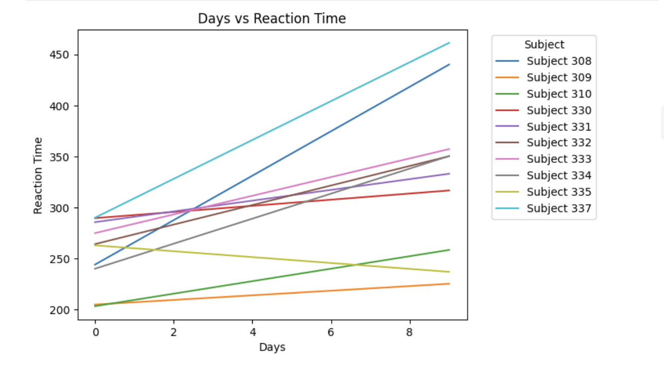
plt.show()3c. Use the code below to select 10 unique Subject IDs and fit a separate simple linear regression of Reaction on Days for each subject. Plot the fitted regression lines on the same graph. What differences do you observe in the slopes or intercepts across subjects? Write 1–2 sentences explaining what this suggests about individual variability.
import matplotlib.pyplot as plt
import numpy as np

plt.figure()
# Select 10 unique subjects
subjects = sleep_study_data["Subject"].unique()[:10]
for subject in subjects:
    subset = sleep_study_data[sleep_study_data["Subject"] == subject]

    # Only fit if enough observations
    if len(subset) > 1:
        m, b = np.polyfit(subset["Days"], subset["Reaction"], 1)

        x_vals = np.linspace(
            subset["Days"].min(),
            subset["Days"].max(),
            100)
        y_vals = m * x_vals + b
        plt.plot(x_vals, y_vals, label=f"Subject {subject}")

plt.xlabel("_________")
plt.ylabel("___________")
plt.title("___________")
plt.legend(title="Subject", bbox_to_anchor=(1.05, 1))
plt.show()Question 4 - Individual Subject Models (2 points)
4a. Subset the data to include only observations for Subject 308 only. Create a scatterplot of Reaction versus Days and overlay the fitted simple linear regression line.
import matplotlib.pyplot as plt
import numpy as np

subset = sleep_study_data[sleep_study_data["Subject"] == ___]

# Fit simple linear regression (Reaction ~ Days)
m, b = np.polyfit(subset["Days"], subset["Reaction"], 1)

# Create regression line values
x_vals = np.linspace(subset["Days"].min(), subset["Days"].max(), 100)
y_vals = m * x_vals + b

# Plot
plt.figure()
plt.scatter(subset["Days"], subset["Reaction"], alpha=0.7)
plt.plot(x_vals, y_vals)

plt.xlabel("________")
plt.ylabel("________")
plt.title("________")

# Add equation text on the plot
eq_text = f"Reaction = {m:.2f} * Days + {b:.2f}"
plt.text(
    0.05, 0.95, eq_text,
    transform=plt.gca().transAxes,
    verticalalignment="top")

plt.show()
4b. Now, subset the data to include only observations for Subject 309 only. Create a scatterplot of Reaction versus Days and overlay the fitted simple linear regression line.
import matplotlib.pyplot as plt
import numpy as np

# Subset data for Subject 309
subset = sleep_study_data[sleep_study_data["Subject"] == ____]

# Fit simple linear regression (Reaction ~ Days)
m, b = np.polyfit(subset["Days"], subset["Reaction"], 1)

# Create regression line values
x_vals = np.linspace(subset["Days"].min(), subset["Days"].max(), 100)
y_vals = m * x_vals + b

# Plot
plt.figure()
plt.scatter(subset["Days"], subset["Reaction"], alpha=0.7)
plt.plot(x_vals, y_vals)

plt.xlabel("______")
plt.ylabel("_____")
plt.title("_______")

# Add equation text on the plot
eq_text = f"Reaction = {m:.2f} * Days + {b:.2f}"
plt.text(
    0.05, 0.95, eq_text,
    transform=plt.gca().transAxes,
    verticalalignment="top")

plt.show()
4c. In 1-2 sentences explain What the major differences are between the two equations for each subject. Why do you think that is?
Question 5 - Mixed Effects Model (2 points)
5a. Use the code below to run a mixed-effects model predicting Reaction from Days, including a random intercept for Subject. Use the same fixed effect as in the simple linear model.
import statsmodels.formula.api as smf

# Mixed-effects model with random intercept for Subject
mixed_model = smf.mixedlm(
    "Reaction ~ Days",
    sleep_study_data,
    groups=sleep_study_data["Subject"])

mixed_results = mixed_model.fit()

print(mixed_results.summary())
5b. Use the model summary to identify the population-level fixed effects and the subject-specific random intercept effects. In 2–3 sentences, describe how the intercept varies across subjects.
5c. Use the code below to extract and display the subject-specific random intercept effects from the mixed-effects model. What do these values represent? In 2–3 sentences, explain how these subject-level deviations modify the overall intercept and what this tells you about individual baseline reaction times.
random_effects = mixed_results.random_effects
for Subject, effect in random_effects.items():
print(f"Subject: {Subject}, Random Intercept: {effect.values[0]:.3f}")Question 6 - Subject Comparisons (2 points)
6a. Use the mixed-effects model and the code below (not the SLR model) to compare two specific subjects 371 and 337 by plotting their subject-specific regression lines.
import statsmodels.formula.api as smf
import numpy as np
import matplotlib.pyplot as plt

# Fit mixed model
mixed_model = smf.mixedlm(
    "Reaction ~ Days",
    sleep_study_data,
    groups=sleep_study_data["Subject"])

mixed_results = mixed_model.fit()

# Fixed effects
fixed_intercept = mixed_results.fe_params["Intercept"]
fixed_slope = mixed_results.fe_params["Days"]

# Extract random intercepts
random_effects = mixed_results.random_effects

# Choose subjects
subject_1 = ___
subject_2 = ___

# Subject-specific intercepts
intercept_1 = fixed_intercept + random_effects[subject_1].values[0]
intercept_2 = fixed_intercept + random_effects[subject_2].values[0]

# X values
x_vals = np.linspace(
    sleep_study_data["Days"].min(),
    sleep_study_data["Days"].max(),
    100)

# Predicted lines
y_1 = intercept_1 + fixed_slope * x_vals
y_2 = intercept_2 + fixed_slope * x_vals

plt.figure()

# Plot lines
plt.plot(x_vals, y_1, linewidth=2, label=f"Subject {subject_1}")
plt.plot(x_vals, y_2, linewidth=2, label=f"Subject {subject_2}")

plt.xlabel("______")
plt.ylabel("______")
plt.title("______")

# Add equations to plot
eq1 = f"S371: Reaction = {intercept_1:.2f} + {fixed_slope:.2f}*Days"
eq2 = f"S337: Reaction = {intercept_2:.2f} + {fixed_slope:.2f}*Days"

plt.text(0.02, 0.95, eq1, transform=plt.gca().transAxes, verticalalignment="top")
plt.text(0.02, 0.88, eq2, transform=plt.gca().transAxes, verticalalignment="top")

plt.legend()
plt.show()
6b. Write 1-2 sentences on what you notice about the differences between the two lines.