Introduction to Time Series
Project Objectives
This project will introduce you to the essential steps of preparing time series data for analysis and forecasting. Time series data requires special attention during the cleaning and transformation process before applying any machine learning method. You will learn how to handle common challenges such as missing values and repeated timestamps to prepare data for modeling.
|
This guide was originally created as a seminar project, so you may notice it follows a question-and-answer format. Even so, it should still serve as a helpful resource to guide you through the process of building your own model. Use 4 cores if you want to replicate this project in Anvil. |
Introduction
“Climate is what we expect, weather is what we get.” – Mark Twain
Everyone is talking about climate change—but what does the data actually say? In this project, you will explore over 18 years of daily weather from Indianapolis and investigate how climate patterns are shifting over time. Of course, the data will not be a clean, pre-packaged dataset. Real data is messy. Some days are missing. Some values use symbols like "T" for trace amounts (small amounts close to 0) or "M" for missing entries. Before we can analyze trends or train a forecasting model, we will need to clean and prepare the data.
This dataset comes from National Oceanic and Atmospheric Administration (NOAA) Local Climatological Data and includes variables such as daily temperature, precipitation, humidity, wind speed, and snowfall for Indianapolis.
These are the key environmental indicators we will work with:
-
DailyAverageDryBulbTemperature: Average air temperature -
DailyMaximumDryBulbTemperatureandDailyMinimumDryBulbTemperature: Max and Min Air Temperature for the day -
DailyPrecipitation: Rainfall or melted snow (inches) -
DailyAverageRelativeHumidity: Moisture in the air -
DailyAverageWindSpeed: Wind patterns (mph) -
DailySnowfall: Snow accumulation (inches)
Why do we need to use time series analysis for this data?
Time series methods are specifically designed to work with data where observations are collected at consistent intervals—like daily, weekly, or monthly so we can understand how things change over time and make predictions about the future. This dataset is a good for time series analysis because it tracks temperature and other weather variables on a daily basis over 18+ years.
In this case, we’re interested in uncovering patterns in climate data, such as:
-
Seasonal trends (e.g., warmer summers, colder winters)
-
Long-term trends (e.g., gradual increase in temperature due to climate change),
-
Short-term fluctuations (e.g., sudden cold snaps or heatwaves),
-
And even forecasting future conditions based on past observations.
However, we cannot jump straight into modeling. Before building a time series model, we must ensure:
-
Dates are properly formatted and consistently spaced,
-
All variables are numeric and in usable units,
-
Missing or trace values (close to 0) are handled appropriately,
-
And the dataset contains no duplicated or skipped dates.
This project will guide you through these foundational steps. By the end, you will not only have a cleaned and structured dataset but you will also understand what makes time series unique, and how to prepare real-world data for powerful forecasting tools like ARIMA or LSTM neural networks.
Time series analysis is a crucial skill in data science, especially for applications in weather forecasting, finance, agriculture, and public health. Mastering the preparation process is your first step toward building models that can anticipate the future.
|
We will ask a series of questions to help you explore the dataset before the deliverables section. These are meant to guide your thinking. The deliverables listed under each question describe what you will need to submit. |
Guided Exploration: Understanding One Year of Weather Data
Before cleaning or modeling time series data, it is essential to understand how the data is structured. Time series methods assume observations occur at regular intervals and that timestamps and measurements are stored in appropriate formats. In this section, you will explore one year of Indianapolis weather data to determine whether it is ready for time series analysis and to identify any structural issues that must be addressed first.
Our focus here is not on fixing the data yet, but on observing how it is recorded: how often measurements occur, whether multiple observations exist per day, and whether variables are stored in usable formats.
Inspecting Data Types and Structure
A critical first step in any time series workflow is verifying data types. Time series analysis relies heavily on correctly formatted datetime variables and numeric measurements. If dates are stored as strings or numeric values are stored as text due to special symbols (such as "T" for trace precipitation or "M" for missing values), many operations—including plotting, resampling, and interpolation—will fail or produce misleading results.
In this dataset, the DATE column must be converted to a datetime object so Python can recognize the temporal ordering of observations. Likewise, temperature, precipitation, and wind variables should be numeric wherever possible.
For reference, Python’s standard built-in data types include:
-
Numeric –
int,float,complex -
Sequence Types –
str,list,tuple -
Mapping Type –
dict -
Boolean –
bool -
Set Types –
set,frozenset -
Binary Types –
bytes,bytearray,memoryview
As you explore the dataset, keep the following guiding questions in mind:
-
What time resolution does the data appear to use?
-
Are observations recorded once per day, or multiple times per day?
-
Do duplicate timestamps exist?
-
Which variables are most relevant for daily weather analysis?
-
Are the current data types appropriate for time series modeling?
Loading and Previewing the Data
To begin, load the 2006 Indianapolis weather dataset and preview the first few rows. This initial glance can reveal missing values, repeated timestamps, or unexpected reporting formats.
import pandas as pd
indy_climatedata_2006 = pd.read_csv(
    "/anvil/projects/tdm/data/noaa_timeseries/indyclimatedata_2006.csv",
    low_memory=False
)
A preview of selected columns is shown below to illustrate the structure of the raw data:
| STATION | DATE | LATITUDE | LONGITUDE | ELEVATION | NAME | REPORT_TYPE | SOURCE | HourlyAltimeterSetting | HourlyDewPointTemperature |
|---|---|---|---|---|---|---|---|---|---|
USW00093819 |
2006-01-01T00:00:00 |
39.72517 |
-86.28168 |
241.1 |
INDIANAPOLIS INTERNATIONAL AIRPORT, IN US |
FM-15 |
335.0 |
1013.5 |
-2.0 |
USW00093819 |
2006-01-01T00:00:00 |
39.72517 |
-86.28168 |
241.1 |
INDIANAPOLIS INTERNATIONAL AIRPORT, IN US |
SOD |
NaN |
NaN |
NaN |
USW00093819 |
2006-01-01T00:00:00 |
39.72517 |
-86.28168 |
241.1 |
INDIANAPOLIS INTERNATIONAL AIRPORT, IN US |
SOM |
NaN |
NaN |
NaN |
USW00093819 |
2006-01-01T00:02:00 |
39.72517 |
-86.28168 |
241.1 |
INDIANAPOLIS INTERNATIONAL AIRPORT, IN US |
FM-16 |
343.0 |
1013.2 |
-2.0 |
USW00093819 |
2006-01-01T00:55:00 |
39.72517 |
-86.28168 |
241.1 |
INDIANAPOLIS INTERNATIONAL AIRPORT, IN US |
FM-15 |
343.0 |
1012.9 |
-2.2 |
Examining Dataset Size and Column Types
Next, examine the size of the dataset and inspect the column names and data types. This information helps determine which variables are likely useful for daily weather analysis and whether any columns will require type conversion or cleaning.
pd.set_option('display.max_rows', None)
print(indy_climatedata_2006.shape)
print(indy_climatedata_2006.dtypes)
Pay particular attention to daily weather variables such as:
-
DailyAverageDryBulbTemperature -
DailyMaximumDryBulbTemperature -
DailyMinimumDryBulbTemperature -
DailyPrecipitation -
DailySnowfall -
DailyAverageRelativeHumidity -
DailyAverageWindSpeed
Many of these variables are numeric and well-suited for analysis, while others, such as precipitation and snowfall, may be stored as objects due to special symbols or missing values.
Converting and Exploring the Date Variable
Time series analysis requires a properly formatted datetime variable. Convert the DATE column using pd.to_datetime() and inspect the result.
indy_climatedata_2006['DATE'] = pd.to_datetime(indy_climatedata_2006['DATE'])
print(indy_climatedata_2006['DATE'].head())
0 2006-01-01 00:00:00
1 2006-01-01 00:00:00
2 2006-01-01 00:00:00
3 2006-01-01 00:02:00
4 2006-01-01 00:55:00
Name: DATE, dtype: datetime64[ns]Notice that multiple observations can occur within the same calendar day, indicating that the dataset contains sub-daily (hourly or event-based) records rather than exactly one row per day.
Understanding the Time Series Granularity
Finally, compare the number of unique calendar dates to the total number of rows. This step confirms whether the dataset represents a true daily time series or a higher-frequency dataset that will need to be aggregated.
indy_climatedata_2006['DATE'].dt.date.nunique()365In 2006, there are 365 unique calendar days in the dataset, but many more rows, confirming that multiple observations exist per day. This observation will directly inform how the data must be transformed before applying daily time series models.
Combining Weather Data Across Multiple Years
In many real-world data science projects, data does not arrive in a single clean file. Instead, it is often spread across multiple years, files, or sources. Building a usable dataset requires carefully combining these pieces into one coherent whole.
In this section, we will assemble nearly two decades of Indianapolis weather data by stacking yearly files into a single DataFrame. Because each file follows the same structure and uses the same column names, they can be safely appended row by row to form one continuous time series.
Combining the data across years allows us to:
-
Examine long-term climate trends in temperature, precipitation, snowfall, and wind,
-
Compare seasonal patterns across different years,
-
Identify gaps, inconsistencies, or incomplete years,
-
Prepare the data for meaningful time series modeling and forecasting.
Understanding the File Structure
Each year of weather data is stored in its own CSV file, following a consistent naming pattern:
-
indyclimatedata_2006.csv -
indyclimatedata_2007.csv -
indyclimatedata_2008.csv -
…
-
indyclimatedata_2024.csv
You can view the available files on ANVIL using the following command:
%%bash
ls /anvil/projects/tdm/data/noaa_timeseries/
Each file contains weather observations for a single year. Our goal is to stack these files together so that the resulting dataset represents a continuous timeline spanning multiple years.
Conceptually, this process is known as appending or stacking data: placing one dataset directly on top of another when they share the same columns. This idea is illustrated below:

As you work through this section, consider the following:
-
Are some years more complete than others?
-
Do all years appear to contain the same number of observations?
-
How might missing or uneven data affect time series analysis?
Loading and Stacking the Yearly Files
To streamline the stacking process, use the function provided below. This function reads each yearly file, adds a year column for tracking, and concatenates all files into a single DataFrame.
import pandas as pd

def load_and_stack_climate_data(start_year=2006, end_year=2024,
                                base_path="/anvil/projects/tdm/data/noaa_timeseries/"):
    dfs = []
    for year in range(start_year, end_year + 1):
        file_path = f"{base_path}indyclimatedata_{year}.csv"
        try:
            df = pd.read_csv(file_path, low_memory=False)
            df['year'] = year
            dfs.append(df)
        except FileNotFoundError:
            print(f"File not found for year {year}: {file_path}")
            continue
    combined_df = pd.concat(dfs, ignore_index=True)
    return combined_df
Use this function to load and combine all available years:
all_years_df_indy_climate = load_and_stack_climate_data()Examining the Combined Dataset
Once all years have been stacked together, examine the size of the combined dataset. This helps verify that the stacking process worked as expected.
all_years_df_indy_climate.shapeNext, break the dataset down by year to see how many rows are recorded for each year:
all_years_df_indy_climate["year"]
    .value_counts()
    .sort_index()
This breakdown reveals whether some years contain more observations than others and provides early insight into data completeness across time.
Focusing on Daily Weather Variables
The full dataset contains many columns, including hourly, daily, and monthly measurements. For the next stages of this project, we will focus on a smaller set of daily weather variables that are most relevant for time series analysis.
Use the code below to filter the dataset to a core set of columns and overwrite the existing DataFrame with this simplified version:
columns_to_keep = [
    "DATE",
    "DailyAverageDryBulbTemperature",
    "DailyMaximumDryBulbTemperature",
    "DailyMinimumDryBulbTemperature",
    "DailyPrecipitation",
    "DailyAverageRelativeHumidity",
    "DailyAverageWindSpeed",
    "DailySnowfall",
    "NAME"
]

all_years_df_indy_climate = all_years_df_indy_climate[columns_to_keep]
Cleaning Daily Weather Data for Time Series Analysis
Before working with time series models, the dataset must be cleaned so that each row represents meaningful daily weather information. This step focuses on selecting relevant variables, removing unusable rows, and ensuring the time variable is stored in a format suitable for time-based analysis.
The variables of interest represent key daily weather conditions, including average, minimum, and maximum temperatures, precipitation, humidity, wind speed, and snowfall. These measurements form the foundation for identifying trends, seasonal patterns, and long-term changes in climate.
Because this project focuses on daily time series analysis, the dataset must satisfy two conditions:
-
Each row must contain usable weather measurements
-
The time variable must follow a consistent daily structure
Removing Rows with No Weather Information
In real-world climate data, some rows contain timestamps and location information but no actual weather measurements. These rows do not contribute anything meaningful to analysis or visualization and can introduce misleading patterns if left in the dataset.
When removing empty rows, it is important to focus only on weather-related columns. Columns such as DATE and NAME should be excluded from this check, since their presence alone does not indicate that useful data exists for a given day.
The goal is to remove rows where all weather measurements are missing, while retaining rows that contain at least one recorded weather value.
cols_to_check = [
    col for col in all_years_df_indy_climate.columns
    if col not in ["DATE", "NAME"]
]

all_years_df_indy_climate = (
    all_years_df_indy_climate
    .dropna(subset=cols_to_check, how="all")
)

all_years_df_indy_climate.head()
A preview of the cleaned data is shown below. Notice that each remaining row contains at least one recorded weather measurement, even if some individual values are still missing or marked as trace amounts.
| DATE | DailyAverageDryBulbTemperature | DailyMaximumDryBulbTemperature | DailyMinimumDryBulbTemperature | DailyPrecipitation | DailyAverageRelativeHumidity | DailyAverageWindSpeed | DailySnowfall | NAME |
|---|---|---|---|---|---|---|---|---|
2006-01-01T00:00:00 |
4.5 |
10.6 |
-1.7 |
0.0 |
74.0 |
5.1 |
0.0 |
INDIANAPOLIS INTERNATIONAL AIRPORT, IN US |
2006-01-02T00:00:00 |
13.3 |
18.3 |
8.3 |
6.6 |
89.0 |
4.9 |
0.0 |
INDIANAPOLIS INTERNATIONAL AIRPORT, IN US |
2006-01-03T00:00:00 |
7.0 |
8.3 |
5.6 |
0.5 |
96.0 |
NaN |
0.0 |
INDIANAPOLIS INTERNATIONAL AIRPORT, IN US |
2006-01-04T00:00:00 |
6.4 |
10.0 |
2.8 |
T |
87.0 |
7.7 |
0.0 |
INDIANAPOLIS INTERNATIONAL AIRPORT, IN US |
2006-01-05T00:00:00 |
1.7 |
3.3 |
0.0 |
T |
82.0 |
5.8 |
T |
INDIANAPOLIS INTERNATIONAL AIRPORT, IN US |
Converting DATE to a Datetime Format
Time series analysis requires that the time variable be stored in a datetime format. Converting the DATE column allows Python to correctly interpret ordering, spacing, and calendar-based operations.
all_years_df_indy_climate["DATE"] = pd.to_datetime(
    all_years_df_indy_climate["DATE"]
)

all_years_df_indy_climate.head()
After conversion, the DATE column follows a clean YYYY-MM-DD format, which is appropriate for daily time series analysis.
| DATE | DailyAverageDryBulbTemperature | DailyMaximumDryBulbTemperature | DailyMinimumDryBulbTemperature | DailyPrecipitation | DailyAverageRelativeHumidity | DailyAverageWindSpeed | DailySnowfall | NAME |
|---|---|---|---|---|---|---|---|---|
2006-01-01 |
4.5 |
10.6 |
-1.7 |
0.0 |
74.0 |
5.1 |
0.0 |
INDIANAPOLIS INTERNATIONAL AIRPORT, IN US |
2006-01-02 |
13.3 |
18.3 |
8.3 |
6.6 |
89.0 |
4.9 |
0.0 |
INDIANAPOLIS INTERNATIONAL AIRPORT, IN US |
2006-01-03 |
7.0 |
8.3 |
5.6 |
0.5 |
96.0 |
NaN |
0.0 |
INDIANAPOLIS INTERNATIONAL AIRPORT, IN US |
2006-01-04 |
6.4 |
10.0 |
2.8 |
T |
87.0 |
7.7 |
0.0 |
INDIANAPOLIS INTERNATIONAL AIRPORT, IN US |
2006-01-05 |
1.7 |
3.3 |
0.0 |
T |
82.0 |
5.8 |
T |
INDIANAPOLIS INTERNATIONAL AIRPORT, IN US |
Verifying Dataset Size and Date Coverage
As a final validation step, it is helpful to examine the size of the cleaned dataset and confirm the range of dates it spans. This ensures that no large portions of the timeline were unintentionally removed during cleaning.
print(all_years_df_indy_climate.shape)
print(all_years_df_indy_climate["DATE"].min().date())
print(all_years_df_indy_climate["DATE"].max().date())
(6940, 9)
2006-01-01
2024-12-31
Preparing Climate Data for Time Series Analysis
Time series analysis requires data to be numeric, time-ordered, and indexed in a way that reflects how observations occur over time. Before building forecasting models or creating time-based visualizations, the dataset must be structured so Python can correctly interpret temporal relationships.
This section focuses on two critical preparation steps: setting the date as the time index and ensuring all weather variables are numeric and usable.
Why the Date Index Matters
Many time series operations in Python rely on the dataframe index rather than column values. One such operation is time-based interpolation, which fills in missing values using the spacing between dates.
If interpolation is attempted before setting the date as the index, Python cannot determine which column represents time. As a result, time-based methods will fail.
For example, attempting to interpolate temperature values without a datetime index produces an error:
DF["DailyAverageDryBulbTemperature"].interpolate(method="time")The error typically indicates that time-weighted interpolation only works when the index is a DatetimeIndex. Without this structure, Python has no information about how observations are ordered in time.
Converting DATE and Setting the Index
To enable time-aware operations, the DATE column must first be converted to a datetime format and then set as the dataframe index.
DF["DATE"] = pd.to_datetime(DF["DATE"])
DF = DF.set_index("DATE")
Once DATE is set as the index, Python recognizes the dataset as time-ordered. Time-based interpolation can now be applied correctly, filling gaps using nearby dates along the timeline.
DF["DailyAverageDryBulbTemperature"].interpolate(
    method="time",
    limit_direction="both"
)
This approach preserves the structure of the time series and avoids introducing artificial jumps or distortions.
Identifying Numeric Columns
Before applying interpolation across the dataset, it is important to identify which columns are numeric. Time-based interpolation should only be applied to numeric variables such as temperature, humidity, and wind speed.
all_years_df_indy_climate.set_index("DATE", inplace=True)

numeric_cols = (
    all_years_df_indy_climate
    .select_dtypes(include="number")
    .columns
)

numeric_cols
Index(['DailyAverageDryBulbTemperature', 'DailyMaximumDryBulbTemperature',
'DailyMinimumDryBulbTemperature', 'DailyAverageRelativeHumidity',
'DailyAverageWindSpeed'],
dtype='object')
These columns represent continuous measurements that vary smoothly over time and are appropriate for interpolation.
Interpolating Missing Values Over Time
With DATE set as the index and numeric columns identified, time-based interpolation can be applied across all numeric variables simultaneously.
all_years_df_indy_climate[numeric_cols] = (
    all_years_df_indy_climate[numeric_cols]
    .interpolate(method="time", limit_direction="both")
)
This ensures that missing values are filled in a way that respects the temporal spacing between observations.
Resetting the Index
After time-based operations are complete, it is often useful to restore DATE as a regular column. This makes the dataframe easier to inspect, merge with other datasets, or visualize using plotting libraries.
all_years_df_indy_climate.reset_index(inplace=True)
all_years_df_indy_climate.head()| DATE | DailyAverageDryBulbTemperature | DailyMaximumDryBulbTemperature | DailyMinimumDryBulbTemperature | DailyPrecipitation | DailyAverageRelativeHumidity | DailyAverageWindSpeed | DailySnowfall | NAME |
|---|---|---|---|---|---|---|---|---|
2006-01-01 |
4.5 |
10.6 |
-1.7 |
0.0 |
74.0 |
5.1 |
0.0 |
INDIANAPOLIS INTERNATIONAL AIRPORT, IN US |
2006-01-02 |
13.3 |
18.3 |
8.3 |
6.6 |
89.0 |
4.9 |
0.0 |
INDIANAPOLIS INTERNATIONAL AIRPORT, IN US |
2006-01-03 |
7.0 |
8.3 |
5.6 |
0.5 |
96.0 |
6.3 |
0.0 |
INDIANAPOLIS INTERNATIONAL AIRPORT, IN US |
2006-01-04 |
6.4 |
10.0 |
2.8 |
T |
87.0 |
7.7 |
0.0 |
INDIANAPOLIS INTERNATIONAL AIRPORT, IN US |
2006-01-05 |
1.7 |
3.3 |
0.0 |
T |
82.0 |
5.8 |
T |
INDIANAPOLIS INTERNATIONAL AIRPORT, IN US |
Handling Trace Values in Weather Data
Weather datasets often include trace values recorded as "T", representing very small amounts of precipitation or snowfall. These values are not numeric and must be addressed before modeling or statistical analysis.
Attempting to convert columns containing "T" directly to floats will result in errors. To resolve this, trace values are replaced with 0 and the columns are then converted to numeric types.
cols_to_fix = [
    "DailyAverageDryBulbTemperature",
    "DailyMaximumDryBulbTemperature",
    "DailyMinimumDryBulbTemperature",
    "DailyPrecipitation",
    "DailyAverageRelativeHumidity",
    "DailyAverageWindSpeed",
    "DailySnowfall"
]

for col in cols_to_fix:
    all_years_df_indy_climate[col] = (
        all_years_df_indy_climate[col]
        .replace("T", 0)
    )

all_years_df_indy_climate[cols_to_fix] = (
    all_years_df_indy_climate[cols_to_fix]
    .astype(float)
)
A final check confirms that no trace values remain in the dataset.
(all_years_df_indy_climate[cols_to_fix] == "T").any()DailyAverageDryBulbTemperature False DailyMaximumDryBulbTemperature False DailyMinimumDryBulbTemperature False DailyPrecipitation False DailyAverageRelativeHumidity False DailyAverageWindSpeed False DailySnowfall False dtype: bool
Exploring Climate Trends Over Time
With the data cleaned and properly structured, the next step is to visualize how temperature changes over time. Visualization plays a central role in time series analysis because it allows trends, seasonal patterns, and unusual behavior to emerge before any formal modeling begins.
This section explores daily average temperature across the full time span of the dataset and then zooms in on a single year to examine seasonal dynamics in greater detail.
Converting Daily Temperature to Fahrenheit
The daily average temperature variable is stored in Celsius. For interpretability and consistency with common U.S. weather reporting, the temperature is converted to Fahrenheit and stored as a new column. Keeping the original Celsius values ensures that no information is lost during the transformation.
all_years_df_indy_climate[
    "DailyAverageDryBulbTemperature_Farenheit"
] = (
    all_years_df_indy_climate["DailyAverageDryBulbTemperature"] * 9/5 + 32
)
Visualizing Temperature Across Multiple Years
Plotting daily average temperature from 2006 to 2024 provides a long-term view of climate behavior in Indianapolis. At this scale, individual daily fluctuations blend together, allowing broader patterns to stand out more clearly.
import matplotlib.pyplot as plt
import pandas as pd

all_years_df_indy_climate["DATE"] = pd.to_datetime(
    all_years_df_indy_climate["DATE"]
)

plt.figure(figsize=(12, 6))
plt.plot(
    all_years_df_indy_climate["DATE"],
    all_years_df_indy_climate["DailyAverageDryBulbTemperature_Farenheit"],
    linewidth=1
)

plt.title("Average Daily Temperature in Indianapolis (2006–2024)")
plt.xlabel("Date")
plt.ylabel("Average Temperature (°F)")
plt.xticks(rotation=45)
plt.tight_layout()
plt.show()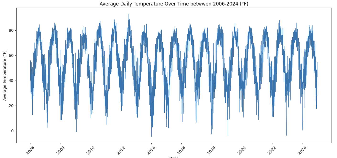
When viewed over many years, several features typically emerge:
-
A strong and repeating seasonal cycle
-
Warmer summers and colder winters
-
Year-to-year variability layered on top of the seasonal pattern
-
Occasional sharp spikes or drops associated with extreme weather events
This visualization helps distinguish long-term structure from short-term noise.
Zooming In on a Single Year
To better understand seasonal behavior, it is useful to focus on a single year. Examining daily average temperature for 2024 allows individual seasonal transitions to be observed more clearly.
At this resolution, patterns such as the following are easier to identify:
-
Temperatures gradually rising from winter into summer
-
Peak temperatures occurring in mid-summer
-
A steady decline from late summer into winter
-
Short-term fluctuations caused by cold snaps, heatwaves, or transitional seasons
Anomalies also become more visible when zoomed in. Brief temperature drops near or below freezing in winter, sudden spikes during transitional months, and irregular spring or fall behavior stand out more clearly at the single-year level.
Why Visual Exploration Matters
Time series visualization provides critical insight into how data behaves over time. Observing strong seasonality suggests the need for models that account for periodic patterns. Long-term trends motivate forecasting approaches that allow gradual change, while anomalies highlight periods that may require special attention.
By examining climate data at both long-term and short-term scales, the dataset begins to tell a story about how temperature evolves over time. This understanding lays the groundwork for the forecasting and modeling techniques introduced next.
Creating Time-Based Features for Seasonal Analysis
With the dataset cleaned, indexed, and visualized, the next step is to extract information directly from the time variable itself. In time series analysis, features derived from the date—such as month, day of year, or day of week—help models recognize recurring patterns and seasonal structure that are not always obvious from raw timestamps alone. This section focuses on creating a month-based feature and using it to summarize long-term seasonal temperature behavior.
Why Time-Based Features Matter
Time-based features allow temporal patterns to be expressed explicitly in the data. Rather than expecting a model to infer seasonality solely from the order of observations, features such as month provide a clear signal about where each observation falls within the yearly cycle.
For climate data, month-based features are especially useful because they align closely with natural seasonal changes:
-
Winter months tend to be colder
-
Summer months tend to be warmer
-
Transitional months often show greater variability
Encoding this information directly makes seasonal structure easier to visualize and model.
Extracting the Month from the DATE Column
To capture seasonal information, the month is extracted from the DATE column and stored as a new variable. The month is represented as a string so it can be treated as a categorical feature in later analyses or models.
all_years_df_indy_climate["MONTH"] = (
    all_years_df_indy_climate["DATE"]
    .dt.month
    .astype(str)
)
This new column assigns each observation a value from "1" through "12", corresponding to January through December.
Calculating Average Temperature by Month
Once the month feature is created, temperatures can be aggregated across all years to examine typical seasonal behavior. Averaging daily temperatures by month reveals long-term patterns that persist year after year.
monthly_avg_temp = (
    all_years_df_indy_climate
    .groupby("MONTH")["DailyAverageDryBulbTemperature_Farenheit"]
    .mean()
    .reset_index()
)

monthly_avg_temp.columns = ["MONTH", "AvgTemp"]
This table summarizes the average temperature associated with each month, smoothing out daily and yearly fluctuations to highlight the overall seasonal cycle.
Visualizing Average Monthly Temperatures
A line plot of average monthly temperatures provides a clear visual representation of seasonal trends. Unlike daily time series plots, this view emphasizes recurring patterns rather than short-term variability.
import matplotlib.pyplot as plt

all_years_df_indy_climate["Month"] = (
    all_years_df_indy_climate["DATE"].dt.month
)

monthly_avg = (
    all_years_df_indy_climate
    .groupby("Month")["DailyAverageDryBulbTemperature_Farenheit"]
    .mean()
    .reset_index()
)

monthly_avg.rename(
    columns={"DailyAverageDryBulbTemperature_Farenheit": "monthly_avg_temp"},
    inplace=True
)

plt.figure(figsize=(10, 5))
plt.plot(
    monthly_avg["Month"],
    monthly_avg["monthly_avg_temp"],
    marker="o"
)

plt.title("Average Monthly Temperature in Indianapolis (Across All Years)")
plt.xlabel("Month")
plt.ylabel("Average Temperature (°F)")
plt.xticks(
    range(1, 13),
    ["Jan", "Feb", "Mar", "Apr", "May", "Jun",
     "Jul", "Aug", "Sep", "Oct", "Nov", "Dec"]
)
plt.grid(True)
plt.tight_layout()
plt.show()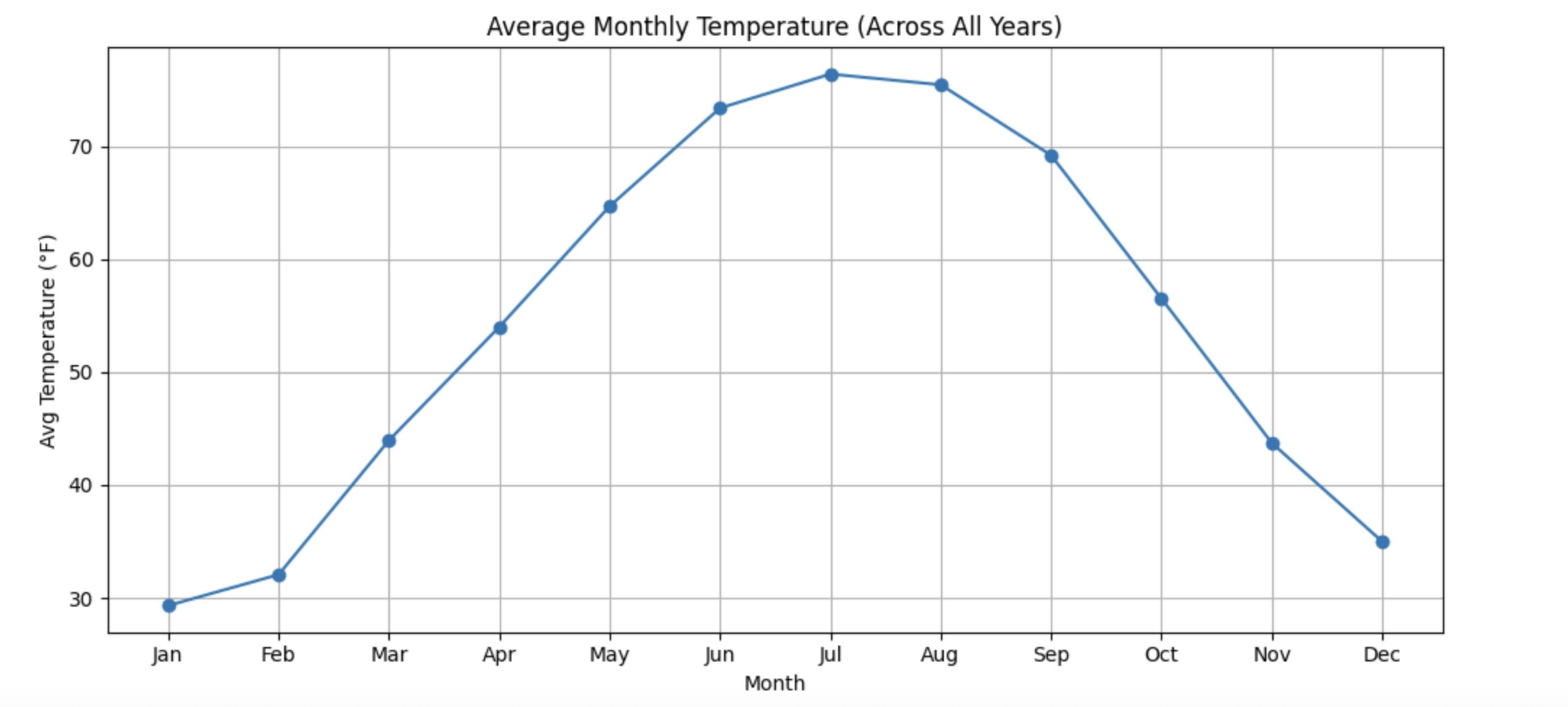
This visualization typically reveals a smooth seasonal curve:
-
Temperatures increase steadily from winter into summer
-
Peak temperatures occur in mid-summer
-
Temperatures decline gradually from late summer into winter
-
Coldest conditions appear in January, with the warmest in July
Connecting Features to Future Modeling
Month-based features play an important role in time series forecasting. Strong seasonal structure suggests that future models should account for periodic behavior rather than treating observations as independent over time.
By explicitly encoding seasonal information and summarizing long-term monthly trends, the dataset becomes better suited for forecasting methods that rely on seasonality, such as SARIMAX models or machine learning approaches that incorporate time-based features.
This step bridges exploratory visualization and formal modeling, ensuring that temporal patterns observed in the data are captured directly in the features used for prediction.