Measuring Model Fit
Introduction
Here we explore various methods for assessing the learning process. We explore how thinking about the output effects how we measure model fit, loss functions (used during the training process), and metrics (used once training is done).
Thinking About the Output
Once you’ve thought about the output, you should have an idea of what kind of data you want to see as output. Maybe its a Boolean, True/False. Maybe its a string, the next expected word in a sentence. Maybe its a probability density function (PDF), "the chance that the variable will be either 1, 2, or 3". Maybe you have an array of numbers that indicate what the expected stock prices should be. Regardless of what your output is, you need a way to measure the performance of your modeling technique. In the context of machine learning, this means you want to measure how well your model has fit the data.
Measuring Unsupervised Output
In a supervised learning setting, you have an output $Y$; but what about in an unsupervised learning situation, where there is no $Y$ output? How can you evaluate the model’s performance when it has no output? This question has been posed by many in the data science world, including in the "machine learning bible", the Introduction to Statistical Learning (see Chapter 12.4, pg 531). The short answer is there is no expert consensus. Here are a few potential workarounds:
-
Assign p-values to clusters
-
Studying the differences between clusters as they get updated at each iteration (are some more stable than others, etc)
-
Validate/confirm with results from a supervised approach
-
Arbitrarily decide before hand how many clusters there should be
-
Don’t bother verifying at all
The rest of this Starter Guide assumes you are using a supervised learning approach.
Measuring Fit During Training: Minimizing The Loss Function
During training, a loss (also called cost) function is used to optimize the model training. This is how the model judges its own performance during training, updates hyperparameters/tuning parameters in response to the loss function, or even implementing early stopping to prevent overfitting.
A loss function is often times naturally chosen; for instance, if we are classifying images where there is only possible label to apply, we would use categorical cross entropy (also known as "softmax loss" because it is the same as the softmax activation function you will learn more of below, generalized as a loss function) as the loss function.
Keras offers many different loss functions. You can find the full list here (along with detailed explanations on which one should be used for your project) and we’ve listed the current (as of Fall 2023) ones below:
Probabilistic losses
-
BinaryCrossentropy
-
CategoricalCrossentropy
-
SparseCategoricalCrossentropy
-
Poisson
-
KLDivergence
Regression losses
-
MeanSquaredError
-
MeanAbsoluteError
-
MeanAbsolutePercentageError
-
MeanSquaredLogarithmicError
-
CosineSimilarity
-
Huber
-
LogCosh
Hinge losses for "maximum-margin" classification
-
Hinge
-
SquaredHinge
-
CategoricalHinge
Measuring Fit After Training: Metrics
There are many metrics, or ways to measure, model fit once training is done. Some of the most well known include accuracy, mean squared error (MSE), mean, categorical cross entropy, or AUC (Area Under Curve). How you measure performance is contextual to your problem, and often times there are many ways that might apply.
While you certainly can construct your own metrics, most data science toolkits have metrics already available as classes/methods. For instance, check out Pytorch’s list of metrics.
Metrics are often chosen in the context of the output. For instance, in classification, accuracy is an obvious choice: what percentage of images are classified correctly? Maybe we have multi-label output (that is, a given classification might have more than 1 label that applies to it), in which case we might use categorical cross entropy.
The names of metrics can vary between the various toolkits, so sometimes you will have to dig into the docs and read what metrics come with it, and what they do.
Keras Metrics
Keras has a well developed set of metrics to use for measuring model fit. Below is the list (as of Fall 2023) of metrics:
-
AUC: Approximates the AUC (Area under the curve) of the ROC or PR curves. -
Accuracy: Calculates how often predictions equal labels. -
BinaryAccuracy: Calculates how often predictions match binary labels. -
BinaryCrossentropy: Computes the crossentropy metric between the labels and predictions. -
BinaryIoU: Computes the Intersection-Over-Union metric for class 0 and/or 1. -
CategoricalAccuracy: Calculates how often predictions match one-hot labels. -
CategoricalCrossentropy: Computes the crossentropy metric between the labels and predictions. -
CategoricalHinge: Computes the categorical hinge metric between y_true and y_pred. -
CosineSimilarity: Computes the cosine similarity between the labels and predictions. -
F1Score: Computes F-1 Score. -
FBetaScore: Computes F-Beta score. -
FalseNegatives: Calculates the number of false negatives. -
FalsePositives: Calculates the number of false positives. -
Hinge: Computes the hinge metric between y_true and y_pred. -
IoU: Computes the Intersection-Over-Union metric for specific target classes. -
KLDivergence: Computes Kullback-Leibler divergence metric between y_true and y_pred. -
LogCoshError: Computes the logarithm of the hyperbolic cosine of the prediction error. -
Mean: Computes the (weighted) mean of the given values. -
MeanAbsoluteError: Computes the mean absolute error between the labels and predictions. -
MeanAbsolutePercentageError: Computes the mean absolute percentage error between y_true and y_pred. -
MeanIoU: Computes the mean Intersection-Over-Union metric. -
MeanMetricWrapper: Wraps a stateless metric function with the Mean metric. -
MeanRelativeError: Computes the mean relative error by normalizing with the given values. -
MeanSquaredError: Computes the mean squared error between y_true and y_pred. -
MeanSquaredLogarithmicError: Computes the mean squared logarithmic error between y_true and y_pred. -
MeanTensor: Computes the element-wise (weighted) mean of the given tensors. -
Metric: Encapsulates metric logic and state. -
OneHotIoU: Computes the Intersection-Over-Union metric for one-hot encoded labels. -
OneHotMeanIoU: Computes mean Intersection-Over-Union metric for one-hot encoded labels. -
Poisson: Computes the Poisson score between y_true and y_pred. -
Precision: Computes the precision of the predictions with respect to the labels. -
PrecisionAtRecall: Computes best precision where recall is >= specified value. -
R2Score: Computes R2 score. -
Recall: Computes the recall of the predictions with respect to the labels. -
RecallAtPrecision: Computes best recall where precision is >= specified value. -
RootMeanSquaredError: Computes root mean squared error metric between y_true and y_pred. -
SensitivityAtSpecificity: Computes best sensitivity where specificity is >= specified value. -
SparseCategoricalAccuracy: Calculates how often predictions match integer labels. -
SparseCategoricalCrossentropy: Computes the crossentropy metric between the labels and predictions. -
SparseTopKCategoricalAccuracy: Computes how often integer targets are in the top K predictions. -
SpecificityAtSensitivity: Computes best specificity where sensitivity is >= specified value. -
SquaredHinge: Computes the squared hinge metric between y_true and y_pred. -
Sum: Computes the (weighted) sum of the given values. -
TopKCategoricalAccuracy: Computes how often targets are in the top K predictions. -
TrueNegatives: Calculates the number of true negatives. -
TruePositives: Calculates the number of true positives.
Commonly Used Metrics
| Pardon the dust! More coming soon! |
Confusion Matrices
Confusion matrices are a common way to measure model fit. They can be visualized like so:
| Expected: Positive | Expected: Negative | |
|---|---|---|
Actual: Positive |
|
|
Actual: Negative |
|
|
The perfect confusion matrix is where the False Negative and False Positive are 0. The TP, FN, FP, and TN will all sum to the total amount of predictions. FP is also known as a Type I error. FN is also known as a Type II error.
As an example of a confusion matrix, imagine we have a Convolutional Neural Network model that is making predictions on images of x-rays, and it wants to correctly predict whether the patient has a disease or not. Say we make 100 predictions with our model. Ideally, the True Positive and True Negative cells will sum to 100; if this were the case, that would mean our model got 100% of the predictions correct. It also would mean that the False Negative and False Positive cells would be zero. In this case, let’s imagine that it has 10 True Positive results, or 10 x-rays which had the disease and the model correctly predicted the disease. It also had 100-10=90 True Negative predictions, which were x-rays where the patient did not have the disease and our model correctly guessed it.
However, let’s interpret an example where our model wasn’t perfect. Below you can see an example of our outcome of 100 predictions:
| Expected: Positive | Expected: Negative | |
|---|---|---|
Actual: Positive |
|
|
Actual: Negative |
|
|
Above, our model got 5 (TP) + 25 (TN) = 30 out of 100 predictions correct. It got 40 False Negatives, or x-rays which were actually positive but which our model predicted to be negative. It got 30 False Positives, or x-rays which were negative but which our model predicted to be positive.
For some confusion matrices, they will present the probabilities rather than the total values in each cell. So, referencing the example above, it would look like:
| Expected: Positive | Expected: Negative | |
|---|---|---|
Actual: Positive |
|
|
Actual: Negative |
|
|
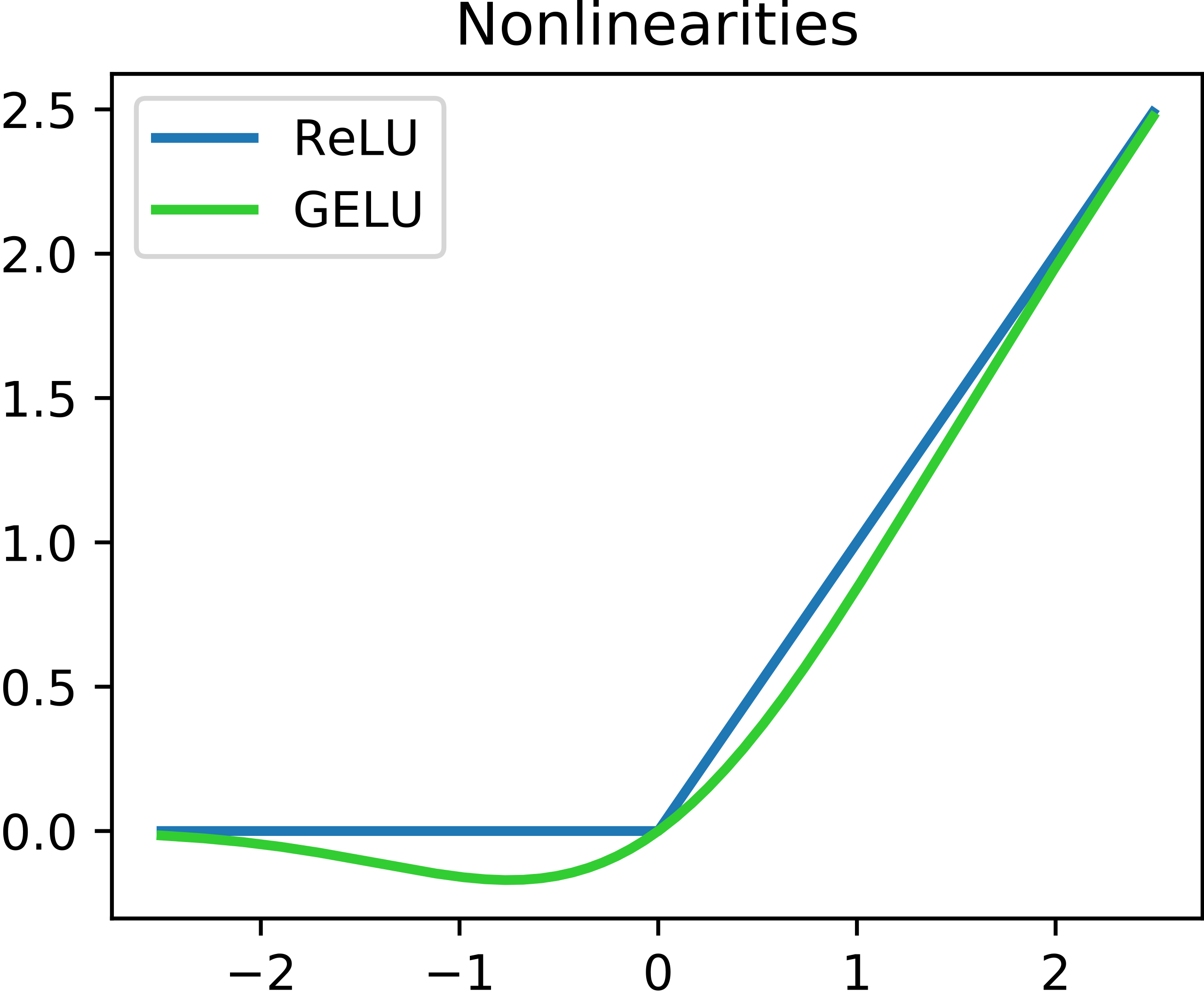
Activation Functions
Activation functions are used for 2 primary purposes:
-
To ensure a nonlinear output
-
To capture complex nonlinearities and interaction effects
They are used especially for neural networks, and are often applied at the end of the training process to produce an output that is guaranteed to produce nonlinear outputs.
Consider one of the most commonly used activation functions for neural nets, ReLU ("Rectified Linear Unit") whose equation is
$ g(z) = (z)_+ = \left\{ \begin{array}{ll} 0 \ \ \ \ \ if \ z<0 \\ z \ \ \ \ \ otherwise \end{array} \right. $
This isn’t the right place to go into detail about this particular activation function, but our source (the Introduction to Statistical Learning (Chapter 10.1) has a much more in depth explanation if you are curious. This will produce a shape like below:
Another function that is commonly used is the sigmoid (sometimes called logistic because it is used for logistic regression) function. The sigmoid function converts linear functions into probabilities between 0 and 1. This is used for binary classification problems ("what is the chance this image has a cat in it") where the output is a binomial probability distribution.
Yet another common function is the softmax function. Softmax is similar to sigmoid, but it differs in that it maps multiple probabilities in the 0 to 1 range. For instance, given an image that might have a dog, cat, or pig in it (so 3 labels) and we know only one of them will be in the image (so this is multi class but not multi label because only 1 label is being applied), our softmax function would return 3 numbers that sum to 1 that represent the odds that the image is a dog [0], cat [1] or pig [2].
Keras Activation Functions
Keras has many common activation functions built into it. You can learn more about the various activation functions on Keras here. Here is the current list of available activation functions (as of Fall 2023):
-
RELU
-
Sigmoid
-
Softmax
-
Softplus
-
Softsign
-
Tanh
-
SELU
-
ELU
-
Exponential
Understanding Cross Validation Metrics
Recall that train, valid and test splits differ in their involvement in training a model. Its important to know that often, training metrics will appear the most positive, validation metrics often the second, and testing metrics are often the lowest, assuming they are all not equal.
The reason why they differ has to do with the training process. Recall that the training data is used for training the model, the validation split is used to verify performance and/or optimize the tuning parameters, and the test split has no involvement in training. In theory, if training goes well, all 3 metrics should be the same (and good in the context of the metric, whether that means a high percentage of accuracy, high $R^2$, etc). In practice, this is rarely the case.
All The Metrics Are Poor
This is indicative of underfitting: your model isn’t able to pick up on the signal as intended. Ensuring you have a healthy train/valid/test ratio and overall size of samples is key. If you have hyper/tuning parameters, try fiddling with those first to see if you can get some intuition on what might help. Make sure you are measuring with the right metrics: for instance, using binary cross entropy when there is multi label output might lead to your model not even making more than 1 prediction like it should. Revisiting your model choice, if you think that maybe this model might not be the best for this particular problem. For instance, if you have incredibly noisy data, a flexible model can accommodate to make a complex model that would be able to pull the signal out of all the noise.
Good Training Metric, Poor Validation Metric
This is often indicative of overfitting. Recall from the Starter Guide page on the bias-variance tradeoff that overfitting occurs when our model is trained to match the training data very well, but generalizes poorly. Why this has occured depends on many things, but sometimes these things can cause it:
-
Not enough training samples
-
Not enough variety in training samples
-
Incredibly complex data with lots of noise
-
Trained for too long
Our Sources
-
Keras, including the metrics page, the loss page and activations page.