Geospatial Analytics using Python and SQL
Route Optimization
Introduction to Route Optimization
Route optimization is the practice of determining the most cost-efficient route, given a start and end location.
A classic computer science example of this is the Traveling Salesman Problem. In this scenario, rhe travelling salesman problem asks the following question: "Given a list of cities and the distances between each pair of cities, what is the shortest possible route that visits each city exactly once and returns to the origin city?" It is an NP-hard problem in combinatorial optimization, important in theoretical computer science and operations research. Please see below for an example of the traveling salesman problem:
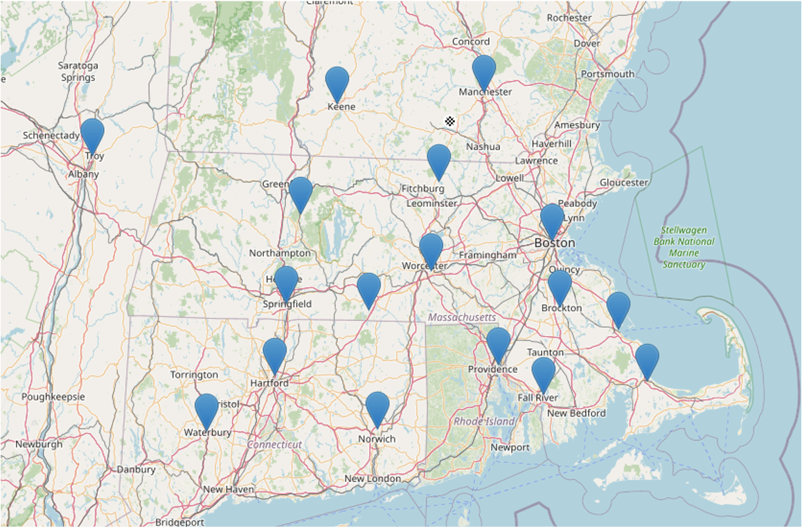
Imagine you are a corporate sales representative for the Northeast. You need to travel to many cities to sell your company’s products, as your salary is based solely on commission. Given the vast size of your sales region, you would like to find the most optimal way to visit all your clients and prospective clients.
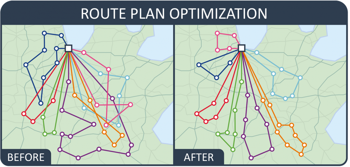
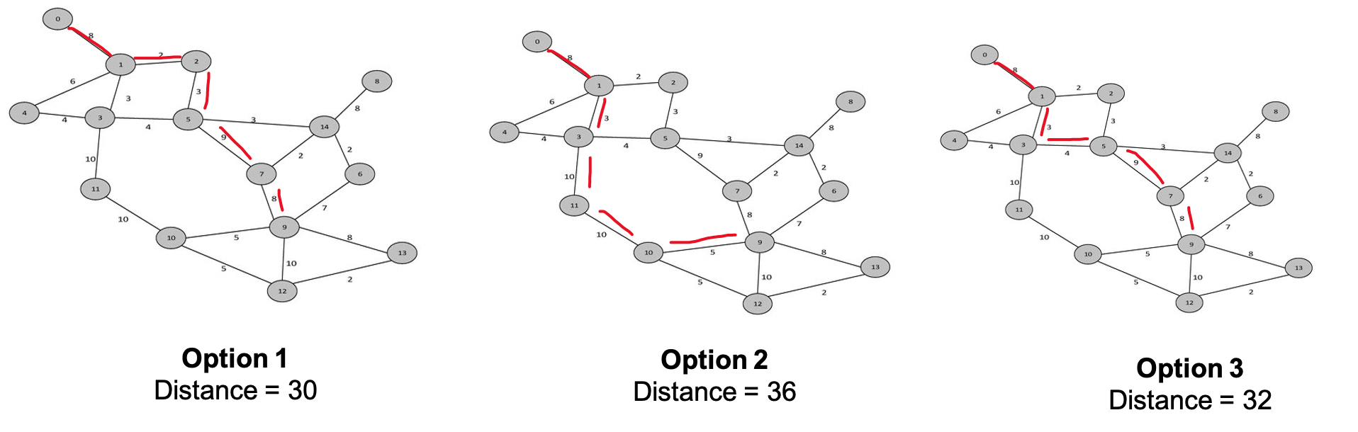
Without route optimization (i.e., shortest distance/least time between all cities in our sales representative’s route), a potential route could look like this:
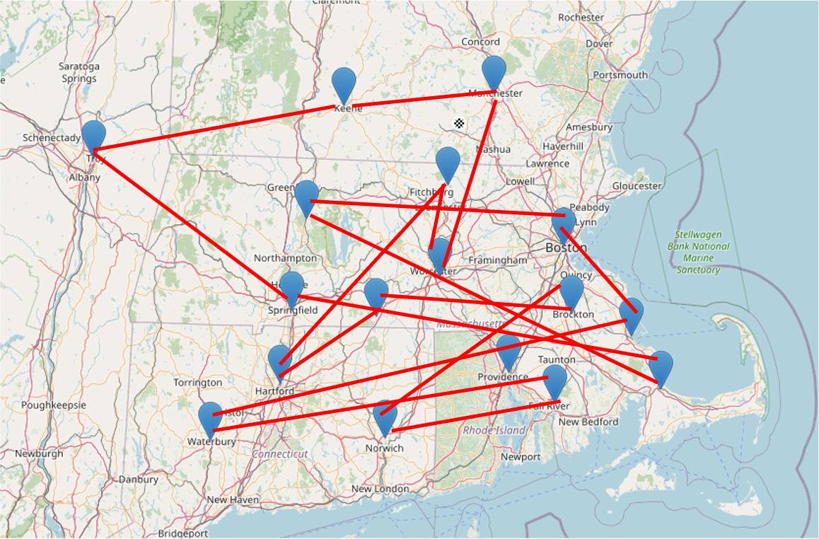
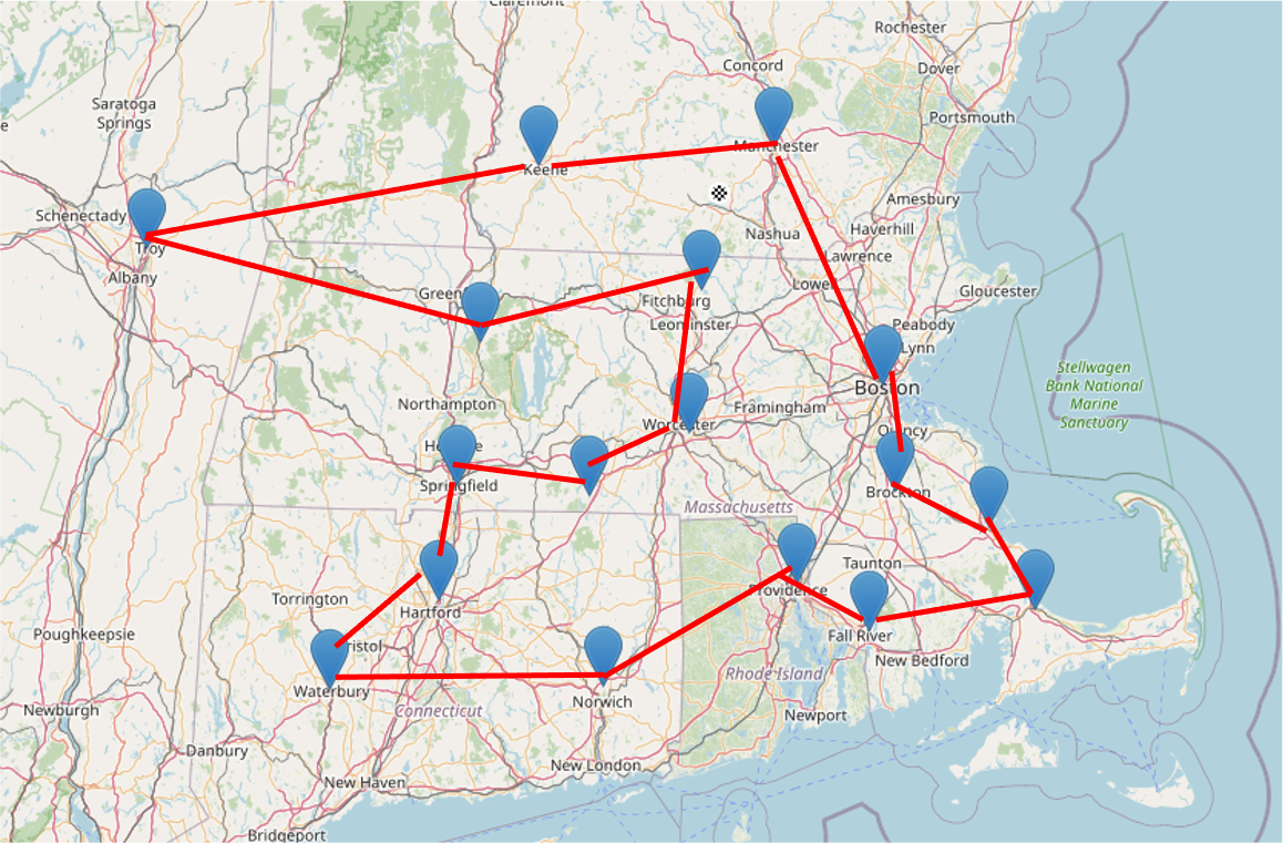
Notice how inefficient the route is. There is a degree of "zig-zagging" occurring, which will cost the sales representative more in gas and time spent. Let’s try adjusting the order of the cities by optimizing for the shortest distance driven—maximizing our representative’s time to see the most clients possible, in a timely manner:
Applications of Routing and Route Optimization
Many different industries, companies, etc. use routing in varying degrees to help their bottom line, and make customers' and employees' lives easier. For example:
-
Ride-sharing, autonomous vehicles, traffic
-
Determining routes, avoiding traffic jams, etc.
-
-
Emergency services and non-emergency medical transport
-
Fastest route to get from dispatch to patient, and to medical care
-
-
Public transit
-
Fleet-level optimization problem on the most efficient routes (i.e., gas and time as optimization constraint) to serve the most number of riders possible
-
-
Supply chain
-
Optimizing a delivery driver’s route to deliver the most number of packages, as quickly as possible
-
Ethics Soapbox
A problem with this approach is unequal access to street addresses. Something we often don’t think about. As explained in Deirdre Mask’s The Address Book, a non-insignificant share of West Virginia and some rural parts of the U.S., as well as developing nations, lack street addresses. How can you route EMS/police to these locations? If you’re interested in equitable access to street addresses, send me an email ([email protected])! I am involved with a non-profit in this space.
Route Optimization Approaches
Graph-based optimization
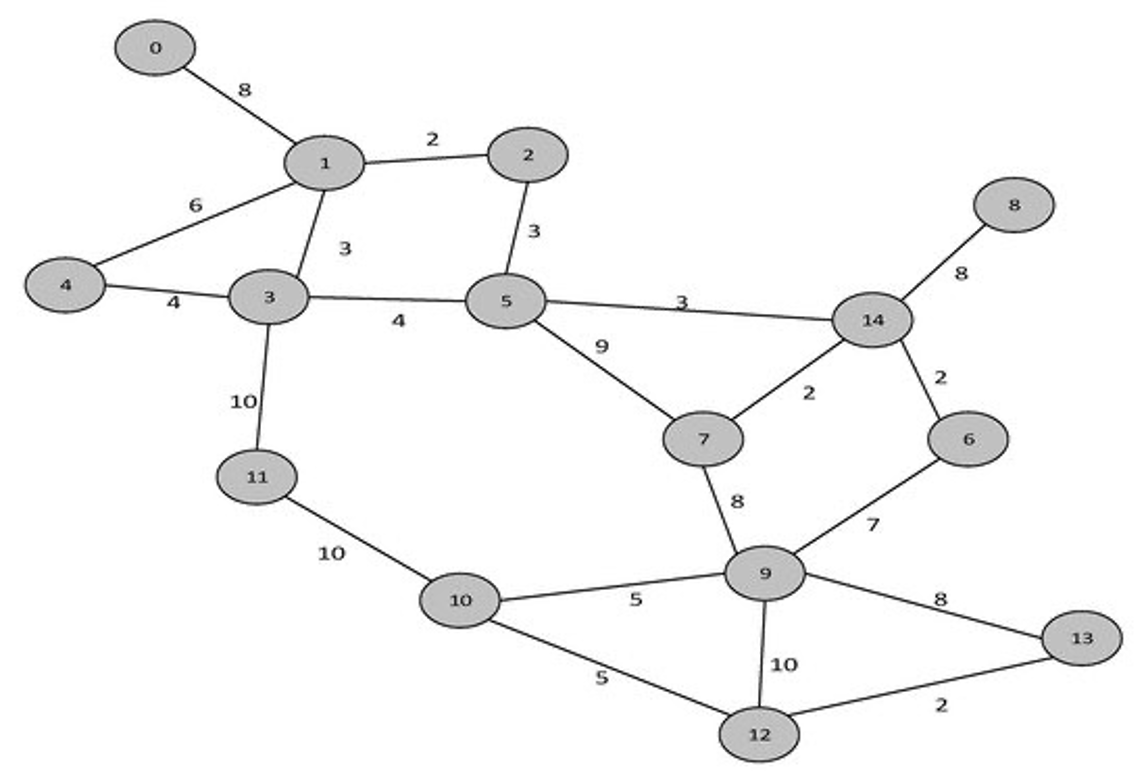
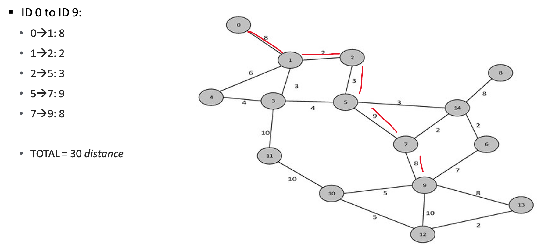
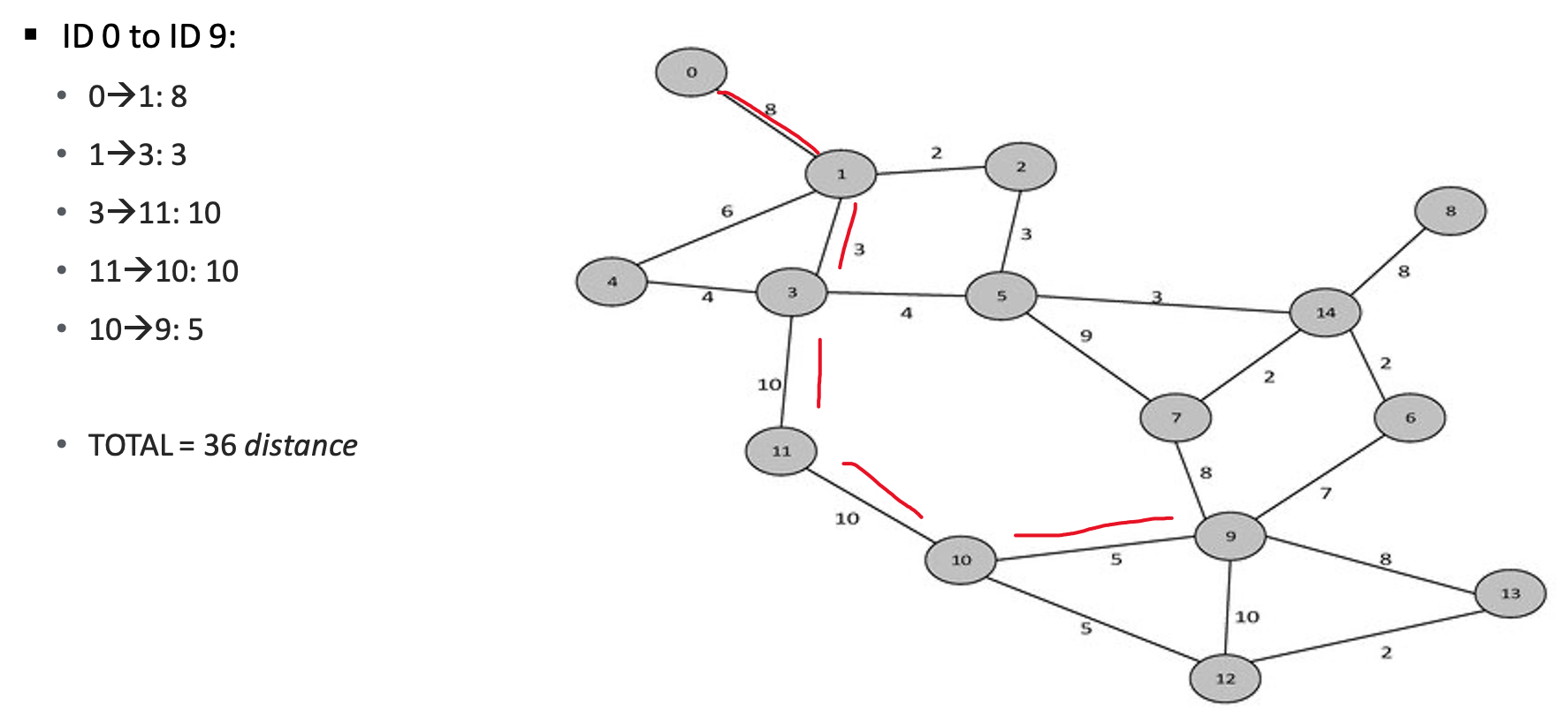
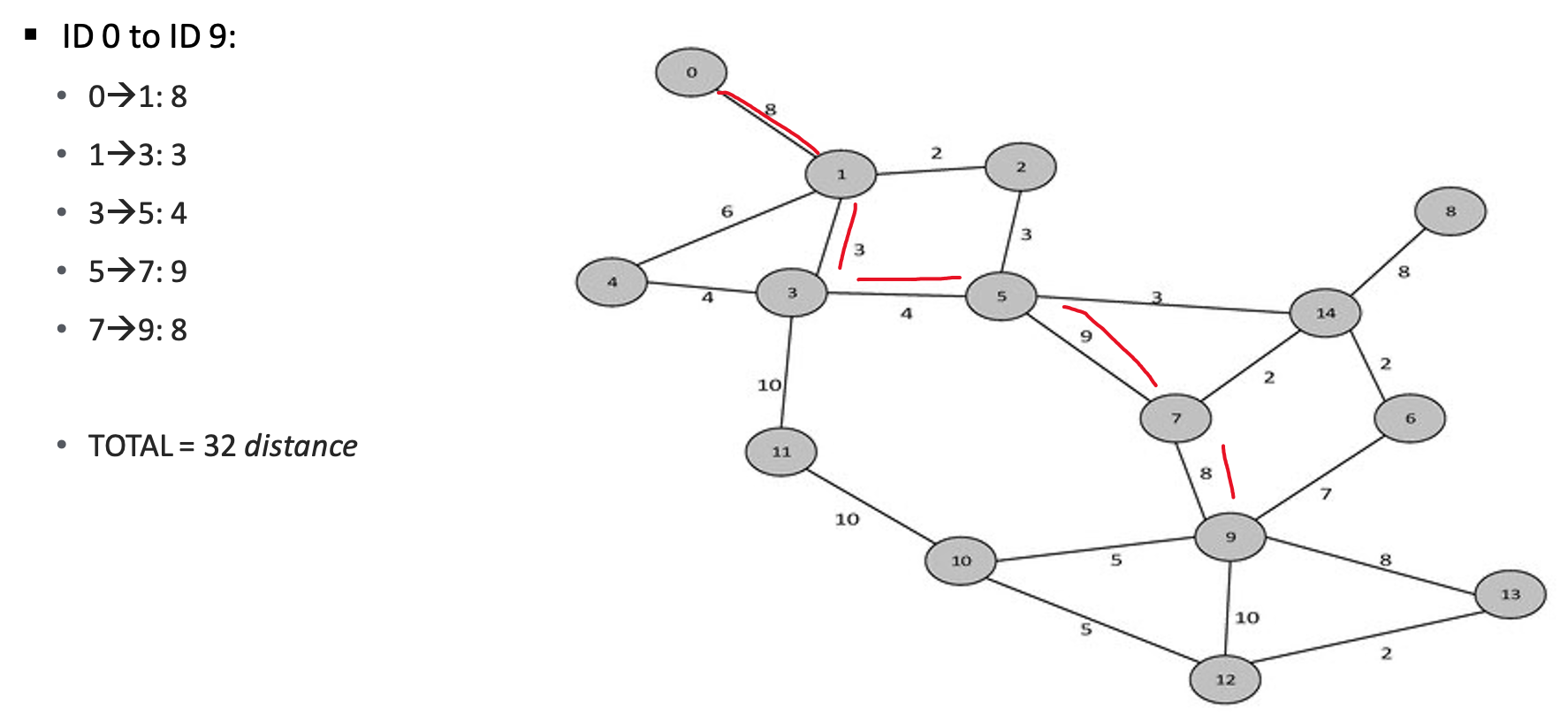
This is the simplest, clearest method for route optimization. It treats everything as a graph, using graph theory and network analysis to compute the shortest path/best route. Each node in the graph below is numbered. Think of it as the node’s ID. A driver must start at 0. What is the shortest path to node ID 9?
Required Packages
*In[106]:*
#mlrose -- see https://stackoverflow.com/a/62354885/9302979
import six
import sys
sys.modules['sklearn.externals.six'] = six
import mlrose
import numpy as np
#Brute Force
from collections import defaultdict
#OR Tools
from ortools.constraint_solver import pywrapcp
from ortools.constraint_solver import routing_enums_pb2
import math
*Out[106]:*
/Users/gould29/opt/anaconda3/envs/honr490/lib/python3.7/site-packages/ipykernel/ipkernel.py:283: DeprecationWarning: `should_run_async` will not call `transform_cell` automatically in the future. Please pass the result to `transformed_cell` argument and any exception that happen during thetransform in `preprocessing_exc_tuple` in IPython 7.17 and above.
  and should_run_async(code)
1. mlrose Solution
towardsdatascience.com/solving-travelling-salesperson-problems-with-python-5de7e883d847
The steps required to solve this problem are the same as those used to
solve any optimization problem in mlrose. Specificially: 1. Define a
fitness function object. 2. Define an optimization problem object. 3.
Select and run a randomized optimization algorithm.
For the TSP in the example, the goal is to find the shortest tour of the
eight cities. As a result, the fitness function should calculate the
total length of a given tour. This is the fitness definition used in
mlrose’s pre-defined TravellingSales() class.
The TSPOpt() optimization problem class assumes, by default, that the
TravellingSales() class is used to define the fitness function for a
TSP. As a result, if the TravellingSales() class is to be used to
define the fitness function object, then this step can be skipped.
However, it is also possible to manually define the fitness function
object, if so desired.
To initialize a fitness function object for the TravellingSales()
class, it is necessary to specify either the (x, y) coordinates of all
the cities or the distances between each pair of cities for which travel
is possible. If the former is specified, then it is assumed that travel
between each pair of cities is possible and that the distance between
the pairs of cities is the Euclidean distance.
If we choose to specify the coordinates, then these should be input as
an ordered list of pairs (where pair i specifies the coordinates of
city i), as follows:
*In[5]:*
Create list of city coordinates
coords_list = [(1, 1), (4, 2), (5, 2), (6, 4), (4, 4), (3, 6), (1, 5), (2, 3)] # Initialize fitness function object using coords_list fitness_coords = mlrose.TravellingSales(coords = coords_list)
Alternatively, if we choose to specify the distances, then these should be input as a list of triples giving the distances, d, between all pairs of cities, u and v, for which travel is possible, with each triple in the form (u, v, d).
The order in which the cities is specified does not matter (i.e., the distance between cities 1 and 2 is assumed to be the same as the distance between cities 2 and 1), and so each pair of cities need only be included in the list once.
Using the distance approach, the fitness function object can be initialized as follows:
*In[6]:*
Create list of distances between pairs of cities
dist_list = [(0, 1, 3.1623), (0, 2, 4.1231), (0, 3, 5.8310), (0, 4, 4.2426), \ (0, 5, 5.3852), (0, 6, 4.0000), (0, 7, 2.2361), (1, 2, 1.0000), \ (1, 3, 2.8284), (1, 4, 2.0000), (1, 5, 4.1231), (1, 6, 4.2426), \ (1, 7, 2.2361), (2, 3, 2.2361), (2, 4, 2.2361), (2, 5, 4.4721), \ (2, 6, 5.0000), (2, 7, 3.1623), (3, 4, 2.0000), (3, 5, 3.6056), \ (3, 6, 5.0990), (3, 7, 4.1231), (4, 5, 2.2361), (4, 6, 3.1623), \ (4, 7, 2.2361), (5, 6, 2.2361), (5, 7, 3.1623), (6, 7, 2.2361)]
Initialize fitness function object using dist_list
fitness_dists = mlrose.TravellingSales(distances = dist_list)
If both a list of coordinates and a list of distances are specified in initializing the fitness function object, then the distance list will be ignored.
Define an Optimization Problem Object
As mentioned previously, the most efficient approach to solving a TSP in
mlrose is to define the optimization problem object using the TSPOpt()
optimization problem class.
If a fitness function has already been manually defined, as demonstrated
in the previous step, then the only additional information required to
initialize a TSPOpt() object are the length of the problem (i.e. the
number of cities to be visited on the tour) and whether our problem is a
maximization or a minimization problem.
In our example, we want to solve a minimization problem of length 8. If
we use the fitness_coords fitness function defined above, we can
define an optimization problem object as follows:
*In[7]:*
problem_fit = mlrose.TSPOpt(length = 8, fitness_fn = fitness_coords,
                            maximize=False)
Alternatively, if we had not previously defined a fitness function (and
we wish to use the TravellingSales() class to define the fitness
function), then this can be done as part of the optimization problem
object initialization step by specifying either a list of coordinates or
a list of distances, instead of a fitness function object, similar to
what was done when manually initializing the fitness function object.
In the case of our example, if we choose to specify a list of coordinates, in place of a fitness function object, we can initialize our optimization problem object as:
*In[9]:*
coords_list = [(1, 1), (4, 2), (5, 2), (6, 4), (4, 4), (3, 6),
               (1, 5), (2, 3)]
problem_no_fit = mlrose.TSPOpt(length = 8, coords = coords_list,
                               maximize=False)
As with manually defining the fitness function object, if both a list of coordinates and a list of distances are specified in initializing the optimization problem object, then the distance list will be ignored. Furthermore, if a fitness function object is specified in addition to a list of coordinates and/or a list of distances, then the list of coordinates/distances will be ignored.
Select and Run a Randomized Optimization Algorithm
Once the optimization object is defined, all that is left to do is to select a randomized optimization algorithm and use it to solve our problem.
This time, suppose we wish to use a genetic algorithm with the default
parameter settings of a population size (pop_size) of 200, a mutation
probability (mutation_prob) of 0.1, a maximum of 10 attempts per step
(max_attempts) and no limit on the maximum total number of iteration
of the algorithm (max_iters).
*In[10]:*
Solve problem using the genetic algorithm
best_state, best_fitness = mlrose.genetic_alg(problem_fit, random_state = 2) print('The best state found is: ', best_state) print('The fitness at the best state is: ', best_fitness)
*Out[10]:*
The best state found is:  [1 3 4 5 6 7 0 2]
The fitness at the best state is:  18.89580466036301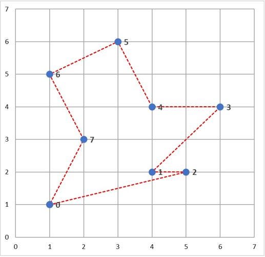
Increasing the maximum number of attempts per step to 100 and increasing the mutation probability to 0.2, yields a tour with a total length of 17.343 units.
*In[11]:*
Solve problem using the genetic algorithm
best_state, best_fitness = mlrose.genetic_alg(problem_fit, mutation_prob = 0.2, max_attempts = 100, random_state = 2) print('The best state found is: ', best_state) print('The fitness at the best state is: ', best_fitness)
*Out[11]:*
The best state found is:  [7 6 5 4 3 2 1 0]
The fitness at the best state is:  17.34261754766733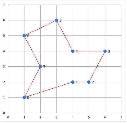
But wait, what is a Genetic Algorithm? Genetic Algorithm Optimization techniques are the techniques used to discover the best solution out of all the possible solutions available under the constraints present. The genetic algorithm is one such optimization algorithm built based on the natural evolutionary process of our nature.

2. Brute-Force (Dijkstra)
benalexkeen.com/implementing-djikstras-shortest-path-algorithm-with-python/
Djikstra’s algorithm is a path-finding algorithm, like those used in
routing and navigation.
We will be using it to find the shortest path between two nodes in a graph.
It fans away from the starting node by visiting the next node of the lowest weight and continues to do so until the next node of the lowest weight is the end node.
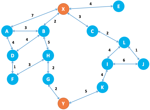
We’ll go work through with an example, let’s say we want to get from X to Y in the graph below with the smallest weight possible. The weights in this example are given by the numbers on the edges between nodes.
Here is what our graph looks like:
We’ll start by constructing this graph in python:
*In[28]:*
class Graph():
    def __init__(self):
        """
        self.edges is a dict of all possible next nodes
        e.g. {'X': ['A', 'B', 'C', 'E'], ...}
        self.weights has all the weights between two nodes,
        with the two nodes as a tuple as the key
        e.g. {('X', 'A'): 7, ('X', 'B'): 2, ...}
        """
        self.edges = defaultdict(list)
        self.weights = {}
    def add_edge(self, from_node, to_node, weight):
        # Note: assumes edges are bi-directional
        self.edges[from_node].append(to_node)
        self.edges[to_node].append(from_node)
        self.weights[(from_node, to_node)] = weight
        self.weights[(to_node, from_node)] = weight
*In[31]:*
graph = Graph()*In[32]:*
#Define Edges and Add to Graph
edges = [
    ('X', 'A', 7),
    ('X', 'B', 2),
    ('X', 'C', 3),
    ('X', 'E', 4),
    ('A', 'B', 3),
    ('A', 'D', 4),
    ('B', 'D', 4),
    ('B', 'H', 5),
    ('C', 'L', 2),
    ('D', 'F', 1),
    ('F', 'H', 3),
    ('G', 'H', 2),
    ('G', 'Y', 2),
    ('I', 'J', 6),
    ('I', 'K', 4),
    ('I', 'L', 4),
    ('J', 'L', 1),
    ('K', 'Y', 5),
]
for edge in edges:
    graph.add_edge(*edge)
Now we need to implement our algorithm.
At our starting node (X), we have the following choice:
-
Visit A next at a cost of 7
-
Visit B next at a cost of 2
-
Visit C next at a cost of 3
-
Visit E next at a cost of 4
We choose the lowest cost option, to visit node B at a cost of 2. We then have the following options:
-
Visit A from X at a cost of 7
-
Visit A from B at a cost of (2 + 3) = 5
-
Visit D from B at a cost of (2 + 4) = 6
-
Visit H from B at a cost of (2 + 5) = 7
-
Visit C from X at a cost of 3
-
Visit E from X at a cost of 4
The next lowest cost item is visiting C from X, so we try that and then we are left with the above options, as well as:
-
Visit L from C at a cost of (3 + 2) = 5
Next we would visit E from X as the next lowest cost is 4.
For each destination node that we visit, we note the possible next destinations and the total weight to visit that destination. If a destination is one we have seen before and the weight to visit is lower than it was previously, this new weight will take its place. For example
-
Visiting A from X is a cost of 7
-
But visiting A from X via B is a cost of 5
-
Therefore we note that the shortest route to X is via B
We only need to keep a note of the previous destination node and the total weight to get there.
We continue evaluating until the destination node weight is the lowest total weight of all possible options.
In this trivial case it is easy to work out that the shortest path will be: \(X -> B -> H -> G -> Y\)
For a total weight of 11.
In this case, we will end up with a note of:
-
The shortest path to Y being via G at a weight of 11
-
The shortest path to G is via H at a weight of 9
-
The shortest path to H is via B at weight of 7
-
The shortest path to B is directly from X at weight of 2
And we can work backwards through this path to get all the nodes on the shortest path from X to Y.
Once we have reached our destination, we continue searching until all possible paths are greater than 11; at that point we are certain that the shortest path is 11.
*In[33]:*
def dijsktra(graph, initial, end):
    # shortest paths is a dict of nodes
    # whose value is a tuple of (previous node, weight)
    shortest_paths = {initial: (None, 0)}
    current_node = initial
    visited = set()
    while current_node != end:
        visited.add(current_node)
        destinations = graph.edges[current_node]
        weight_to_current_node = shortest_paths[current_node][1]
        for next_node in destinations:
            weight = graph.weights[(current_node, next_node)] + weight_to_current_node
            if next_node not in shortest_paths:
                shortest_paths[next_node] = (current_node, weight)
            else:
                current_shortest_weight = shortest_paths[next_node][1]
                if current_shortest_weight > weight:
                    shortest_paths[next_node] = (current_node, weight)
        next_destinations = {node: shortest_paths[node] for node in shortest_paths if node not in visited}
        if not next_destinations:
            return "Route Not Possible"
        # next node is the destination with the lowest weight
        current_node = min(next_destinations, key=lambda k: next_destinations[k][1])
    # Work back through destinations in shortest path
    path = []
    while current_node is not None:
        path.append(current_node)
        next_node = shortest_paths[current_node][0]
        current_node = next_node
    # Reverse path
    path = path[::-1]
    return path
*In[34]:*
dijsktra(graph, 'X', 'Y')*Out[34]:*
Here is what our graph looks like:
3. Google OR Tools
*In[35]:*
def create_data_model():
"""Stores the data for the problem."""
data = {}
data['distance_matrix'] = [
[0, 2451, 713, 1018, 1631, 1374, 2408, 213, 2571, 875, 1420, 2145, 1972],
[2451, 0, 1745, 1524, 831, 1240, 959, 2596, 403, 1589, 1374, 357, 579],
[713, 1745, 0, 355, 920, 803, 1737, 851, 1858, 262, 940, 1453, 1260],
[1018, 1524, 355, 0, 700, 862, 1395, 1123, 1584, 466, 1056, 1280, 987],
[1631, 831, 920, 700, 0, 663, 1021, 1769, 949, 796, 879, 586, 371],
[1374, 1240, 803, 862, 663, 0, 1681, 1551, 1765, 547, 225, 887, 999],
[2408, 959, 1737, 1395, 1021, 1681, 0, 2493, 678, 1724, 1891, 1114, 701],
[213, 2596, 851, 1123, 1769, 1551, 2493, 0, 2699, 1038, 1605, 2300, 2099],
[2571, 403, 1858, 1584, 949, 1765, 678, 2699, 0, 1744, 1645, 653, 600],
[875, 1589, 262, 466, 796, 547, 1724, 1038, 1744, 0, 679, 1272, 1162],
[1420, 1374, 940, 1056, 879, 225, 1891, 1605, 1645, 679, 0, 1017, 1200],
[2145, 357, 1453, 1280, 586, 887, 1114, 2300, 653, 1272, 1017, 0, 504],
[1972, 579, 1260, 987, 371, 999, 701, 2099, 600, 1162, 1200, 504, 0],
] # yapf: disable
data['num_vehicles'] = 1
data['depot'] = 0
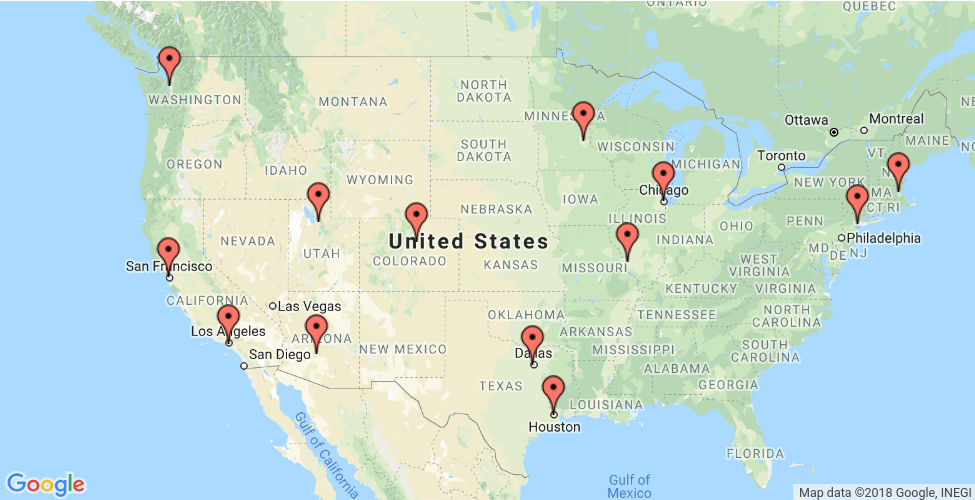
return dataThe distance matrix is an array whose i, j entry is the distance from location i to location j in miles, where the array indices correspond to the locations in the following order:
-
New York - 1. Los Angeles - 2. Chicago - 3. Minneapolis - 4. Denver -
-
Dallas - 6. Seattle - 7. Boston - 8. San Francisco - 9. St. Louis -
-
Houston - 11. Phoenix - 12. Salt Lake City
-
Note: The order of the locations in the distance matrix is arbitrary, and is unrelated to the order of locations in any solution to the TSP.
The data also includes:
-
The number of vehicles in the problem, which is 1 because this is a TSP. (For a vehicle routing problem (VRP), the number of vehicles can be greater than 1.)
-
The depot: the start and end location for the route. In this case, the depot is 0, which corresponds to New York.
Note: Since the routing solver does all computations with integers, the
distance callback must return an integer distance for any two locations.
If any of the entries of data['distance_matrix'] are not integers, you
need to round either the matrix entries, or the return values of the
callback, to integers. See
Scaling
the distance matrix for an example that shows how to avoid problems
caused by rounding error.
Other ways to create the distance matrix
In this example, the distance matrix is explicitly defined in the program. It’s also possible to use a function to calculate distances between locations: for example, the Euclidean formula for the distance between points in the plane. However, it’s still more efficient to pre-compute all the distances between locations and store them in a matrix, rather than compute them at run time. See Example: drilling a circuit board for an example that creates the distance matrix this way.
Another alternative is to use the Google Maps Distance Matrix API to dynamically create a distance (or travel time) matrix for a routing problem. Create the routing model
The following code in the main section of the programs creates the index
manager (manager) and the routing model (routing). The method
manager.IndexToNode converts the solver’s internal indices (which you
can safely ignore) to the numbers for locations. Location numbers
correspond to the indices for the distance matrix.
*In[39]:*
data = create_data_model()
manager = pywrapcp.RoutingIndexManager(len(data['distance_matrix']),
                                       data['num_vehicles'], data['depot'])
routing = pywrapcp.RoutingModel(manager)
The inputs to RoutingIndexManager are:
-
The number of rows of the distance matrix, which is the number of locations (including the depot).
-
The number of vehicles in the problem.
-
The node corresponding to the depot.
Create the distance callback
To use the routing solver, you need to create a distance (or transit) callback: a function that takes any pair of locations and returns the distance between them. The easiest way to do this is using the distance matrix.
The following function creates the callback and registers it with the
solver as transit_callback_index.
*In[40]:*
def distance_callback(from_index, to_index):
    """Returns the distance between the two nodes."""
    # Convert from routing variable Index to distance matrix NodeIndex.
    from_node = manager.IndexToNode(from_index)
    to_node = manager.IndexToNode(to_index)
    return data['distance_matrix'][from_node][to_node]
transit_callback_index = routing.RegisterTransitCallback(distance_callback)
The callback accepts two indices, from_index and to_index, and
returns the corresponding entry of the distance matrix.
Set the cost of travel
The arc cost evaluator tells the solver how to calculate the cost of travel between any two locations—in other words, the cost of the edge (or arc) joining them in the graph for the problem. The following code sets the arc cost evaluator.
In this example, the arc cost evaluator is the transit_callback_index,
which is the solver’s internal reference to the distance callback. This
means that the cost of travel between any two locations is just the
distance between them. However, in general the costs can involve other
factors as well.
You can also define multiple arc cost evaluators that depend on which
vehicle is traveling between locations, using the method
routing.SetArcCostEvaluatorOfVehicle(). For example, if the vehicles
have different speeds, you could define the cost of travel between
locations to be the distance divided by the vehicle’s speed—in other
words, the travel time.
*In[41]:*
routing.SetArcCostEvaluatorOfAllVehicles(transit_callback_index)Set search parameters
The following code sets the default search parameters and a heuristic
method for finding the first solution. The code sets the first solution
strategy to PATH_CHEAPEST_ARC, which creates an initial route for the
solver by repeatedly adding edges with the least weight that don’t lead
to a previously visited node (other than the depot).
*In[44]:*
search_parameters = pywrapcp.DefaultRoutingSearchParameters()
search_parameters.first_solution_strategy = (
    routing_enums_pb2.FirstSolutionStrategy.PATH_CHEAPEST_ARC)
Add the solution printer
The function that displays the solution returned by the solver is shown
below. The function extracts the route from the solution and prints it
to the console. The function displays the optimal route and its
distance, which is given by ObjectiveValue().
*In[45]:*
def print_solution(manager, routing, solution):
    """Prints solution on console."""
    print('Objective: {} miles'.format(solution.ObjectiveValue()))
    index = routing.Start(0)
    plan_output = 'Route for vehicle 0:\n'
    route_distance = 0
    while not routing.IsEnd(index):
        plan_output += ' {} ->'.format(manager.IndexToNode(index))
        previous_index = index
        index = solution.Value(routing.NextVar(index))
        route_distance += routing.GetArcCostForVehicle(previous_index, index, 0)
    plan_output += ' {}\n'.format(manager.IndexToNode(index))
    print(plan_output)
    plan_output += 'Route distance: {}miles\n'.format(route_distance)
Run the Program
*In[46]:*
solution = routing.SolveWithParameters(search_parameters)
if solution:
    print_solution(manager, routing, solution)
*Out[46]:*
Objective: 7293 miles
Route for vehicle 0:
 0 -> 7 -> 2 -> 3 -> 4 -> 12 -> 6 -> 8 -> 1 -> 11 -> 10 -> 5 -> 9 -> 0
Save routes to a list or array
As an alternative to printing the solution directly, you can save the route (or routes, for a VRP) to a list or array. This has the advantage of making the routes available in case you want to do something with them later. For example, you could run the program several times with different parameters and save the routes in the returned solutions to a file for comparison.
*In[48]:*
def get_routes(solution, routing, manager):
    """Get vehicle routes from a solution and store them in an array."""
    # Get vehicle routes and store them in a two dimensional array whose
    # i,j entry is the jth location visited by vehicle i along its route.
    routes = []
    for route_nbr in range(routing.vehicles()):
        index = routing.Start(route_nbr)
        route = [manager.IndexToNode(index)]
    while not routing.IsEnd(index):
        index = solution.Value(routing.NextVar(index))
        route.append(manager.IndexToNode(index))
    routes.append(route)
    return routes
*In[49]:*
routes = get_routes(solution, routing, manager)
# Display the routes.
for i, route in enumerate(routes):
    print('Route', i, route)
*Out[49]:*
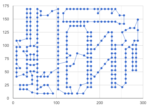
Route 0 [0, 7, 2, 3, 4, 12, 6, 8, 1, 11, 10, 5, 9, 0]2-D Example via OR Tools
This example mimics what we did above, but now using 2-D data. Without a
road network, though. This is an important distinction.
This is what our data look like:
*In[51]:*
def create_data_model():
    """Stores the data for the problem."""
    data = {}
    # Locations in block units
    data['locations'] = [
        (288, 149), (288, 129), (270, 133), (256, 141), (256, 157), (246, 157),
        (236, 169), (228, 169), (228, 161), (220, 169), (212, 169), (204, 169),
        (196, 169), (188, 169), (196, 161), (188, 145), (172, 145), (164, 145),
        (156, 145), (148, 145), (140, 145), (148, 169), (164, 169), (172, 169),
        (156, 169), (140, 169), (132, 169), (124, 169), (116, 161), (104, 153),
        (104, 161), (104, 169), (90, 165), (80, 157), (64, 157), (64, 165),
        (56, 169), (56, 161), (56, 153), (56, 145), (56, 137), (56, 129),
        (56, 121), (40, 121), (40, 129), (40, 137), (40, 145), (40, 153),
        (40, 161), (40, 169), (32, 169), (32, 161), (32, 153), (32, 145),
        (32, 137), (32, 129), (32, 121), (32, 113), (40, 113), (56, 113),
        (56, 105), (48, 99), (40, 99), (32, 97), (32, 89), (24, 89),
        (16, 97), (16, 109), (8, 109), (8, 97), (8, 89), (8, 81),
        (8, 73), (8, 65), (8, 57), (16, 57), (8, 49), (8, 41),
        (24, 45), (32, 41), (32, 49), (32, 57), (32, 65), (32, 73),
        (32, 81), (40, 83), (40, 73), (40, 63), (40, 51), (44, 43),
        (44, 35), (44, 27), (32, 25), (24, 25), (16, 25), (16, 17),
        (24, 17), (32, 17), (44, 11), (56, 9), (56, 17), (56, 25),
        (56, 33), (56, 41), (64, 41), (72, 41), (72, 49), (56, 49),
        (48, 51), (56, 57), (56, 65), (48, 63), (48, 73), (56, 73),
        (56, 81), (48, 83), (56, 89), (56, 97), (104, 97), (104, 105),
        (104, 113), (104, 121), (104, 129), (104, 137), (104, 145), (116, 145),
        (124, 145), (132, 145), (132, 137), (140, 137), (148, 137), (156, 137),
        (164, 137), (172, 125), (172, 117), (172, 109), (172, 101), (172, 93),
        (172, 85), (180, 85), (180, 77), (180, 69), (180, 61), (180, 53),
        (172, 53), (172, 61), (172, 69), (172, 77), (164, 81), (148, 85),
        (124, 85), (124, 93), (124, 109), (124, 125), (124, 117), (124, 101),
        (104, 89), (104, 81), (104, 73), (104, 65), (104, 49), (104, 41),
        (104, 33), (104, 25), (104, 17), (92, 9), (80, 9), (72, 9),
        (64, 21), (72, 25), (80, 25), (80, 25), (80, 41), (88, 49),
        (104, 57), (124, 69), (124, 77), (132, 81), (140, 65), (132, 61),
        (124, 61), (124, 53), (124, 45), (124, 37), (124, 29), (132, 21),
        (124, 21), (120, 9), (128, 9), (136, 9), (148, 9), (162, 9),
        (156, 25), (172, 21), (180, 21), (180, 29), (172, 29), (172, 37),
        (172, 45), (180, 45), (180, 37), (188, 41), (196, 49), (204, 57),
        (212, 65), (220, 73), (228, 69), (228, 77), (236, 77), (236, 69),
        (236, 61), (228, 61), (228, 53), (236, 53), (236, 45), (228, 45),
        (228, 37), (236, 37), (236, 29), (228, 29), (228, 21), (236, 21),
        (252, 21), (260, 29), (260, 37), (260, 45), (260, 53), (260, 61),
        (260, 69), (260, 77), (276, 77), (276, 69), (276, 61), (276, 53),
        (284, 53), (284, 61), (284, 69), (284, 77), (284, 85), (284, 93),
        (284, 101), (288, 109), (280, 109), (276, 101), (276, 93), (276, 85),
        (268, 97), (260, 109), (252, 101), (260, 93), (260, 85), (236, 85),
        (228, 85), (228, 93), (236, 93), (236, 101), (228, 101), (228, 109),
        (228, 117), (228, 125), (220, 125), (212, 117), (204, 109), (196, 101),
        (188, 93), (180, 93), (180, 101), (180, 109), (180, 117), (180, 125),
        (196, 145), (204, 145), (212, 145), (220, 145), (228, 145), (236, 145),
        (246, 141), (252, 125), (260, 129), (280, 133)
    ]  # yapf: disable
    data['num_vehicles'] = 1
    data['depot'] = 0
    return data
def compute_euclidean_distance_matrix(locations):
    """Creates callback to return distance between points."""
    distances = {}
    for from_counter, from_node in enumerate(locations):
        distances[from_counter] = {}
        for to_counter, to_node in enumerate(locations):
            if from_counter == to_counter:
                distances[from_counter][to_counter] = 0
            else:
                # Euclidean distance
                distances[from_counter][to_counter] = (int(
                    math.hypot((from_node[0] - to_node[0]),
                               (from_node[1] - to_node[1]))))
    return distances
def print_solution(manager, routing, solution):
    """Prints solution on console."""
    print('Objective: {}'.format(solution.ObjectiveValue()))
    index = routing.Start(0)
    plan_output = 'Route:\n'
    route_distance = 0
    while not routing.IsEnd(index):
        plan_output += ' {} ->'.format(manager.IndexToNode(index))
        previous_index = index
        index = solution.Value(routing.NextVar(index))
        route_distance += routing.GetArcCostForVehicle(previous_index, index, 0)
    plan_output += ' {}\n'.format(manager.IndexToNode(index))
    print(plan_output)
    plan_output += 'Objective: {}m\n'.format(route_distance)
def main():
    """Entry point of the program."""
    # Instantiate the data problem.
    data = create_data_model()
    # Create the routing index manager.
    manager = pywrapcp.RoutingIndexManager(len(data['locations']),
                                           data['num_vehicles'], data['depot'])
    # Create Routing Model.
    routing = pywrapcp.RoutingModel(manager)
    distance_matrix = compute_euclidean_distance_matrix(data['locations'])
    def distance_callback(from_index, to_index):
        """Returns the distance between the two nodes."""
        # Convert from routing variable Index to distance matrix NodeIndex.
        from_node = manager.IndexToNode(from_index)
        to_node = manager.IndexToNode(to_index)
        return distance_matrix[from_node][to_node]
    transit_callback_index = routing.RegisterTransitCallback(distance_callback)
    # Define cost of each arc.
    routing.SetArcCostEvaluatorOfAllVehicles(transit_callback_index)
    # Setting first solution heuristic.
    search_parameters = pywrapcp.DefaultRoutingSearchParameters()
    search_parameters.first_solution_strategy = (
        routing_enums_pb2.FirstSolutionStrategy.PATH_CHEAPEST_ARC)
    # Solve the problem.
    solution = routing.SolveWithParameters(search_parameters)
    # Print solution on console.
    if solution:
        print_solution(manager, routing, solution)
*In[56]:*
main()*Out[56]:*
Objective: 2790
Route:
 0 -> 1 -> 279 -> 2 -> 278 -> 277 -> 248 -> 247 -> 243 -> 242 -> 241 -> 240 -> 239 -> 238 -> 245 -> 244 -> 246 -> 249 -> 250 -> 229 -> 228 -> 231 -> 230 -> 237 -> 236 -> 235 -> 234 -> 233 -> 232 -> 227 -> 226 -> 225 -> 224 -> 223 -> 222 -> 218 -> 221 -> 220 -> 219 -> 202 -> 203 -> 204 -> 205 -> 207 -> 206 -> 211 -> 212 -> 215 -> 216 -> 217 -> 214 -> 213 -> 210 -> 209 -> 208 -> 251 -> 254 -> 255 -> 257 -> 256 -> 253 -> 252 -> 139 -> 140 -> 141 -> 142 -> 143 -> 199 -> 201 -> 200 -> 195 -> 194 -> 193 -> 191 -> 190 -> 189 -> 188 -> 187 -> 163 -> 164 -> 165 -> 166 -> 167 -> 168 -> 169 -> 171 -> 170 -> 172 -> 105 -> 106 -> 104 -> 103 -> 107 -> 109 -> 110 -> 113 -> 114 -> 116 -> 117 -> 61 -> 62 -> 63 -> 65 -> 64 -> 84 -> 85 -> 115 -> 112 -> 86 -> 83 -> 82 -> 87 -> 111 -> 108 -> 89 -> 90 -> 91 -> 102 -> 101 -> 100 -> 99 -> 98 -> 97 -> 96 -> 95 -> 94 -> 93 -> 92 -> 79 -> 88 -> 81 -> 80 -> 78 -> 77 -> 76 -> 74 -> 75 -> 73 -> 72 -> 71 -> 70 -> 69 -> 66 -> 68 -> 67 -> 57 -> 56 -> 55 -> 54 -> 53 -> 52 -> 51 -> 50 -> 49 -> 48 -> 47 -> 46 -> 45 -> 44 -> 43 -> 58 -> 60 -> 59 -> 42 -> 41 -> 40 -> 39 -> 38 -> 37 -> 36 -> 35 -> 34 -> 33 -> 32 -> 31 -> 30 -> 29 -> 124 -> 123 -> 122 -> 121 -> 120 -> 119 -> 118 -> 156 -> 157 -> 158 -> 173 -> 162 -> 161 -> 160 -> 174 -> 159 -> 150 -> 151 -> 155 -> 152 -> 154 -> 153 -> 128 -> 129 -> 130 -> 131 -> 18 -> 19 -> 20 -> 127 -> 126 -> 125 -> 28 -> 27 -> 26 -> 25 -> 21 -> 24 -> 22 -> 23 -> 13 -> 12 -> 14 -> 11 -> 10 -> 9 -> 7 -> 8 -> 6 -> 5 -> 275 -> 274 -> 273 -> 272 -> 271 -> 270 -> 15 -> 16 -> 17 -> 132 -> 149 -> 177 -> 176 -> 175 -> 178 -> 179 -> 180 -> 181 -> 182 -> 183 -> 184 -> 186 -> 185 -> 192 -> 196 -> 197 -> 198 -> 144 -> 145 -> 146 -> 147 -> 148 -> 138 -> 137 -> 136 -> 135 -> 134 -> 133 -> 269 -> 268 -> 267 -> 266 -> 265 -> 264 -> 263 -> 262 -> 261 -> 260 -> 258 -> 259 -> 276 -> 3 -> 4 -> 0