What Does The Function Mean In The Context Of Data Science?
Introduction
Here we explore the meaning of a function, $ f(x) $ in the context of data science. We will look at the basic equation $Y = f(X) + \epsilon $, how this equation can point us towards our general goal in data science, why reducing error is important, and how to estimate $f$.
The Function $Y = f(X) + \epsilon $
You recall that the output (also called dependent or response variables) is denoted using $ Y $. You will see little $y$ to represent individual outputs of big $Y$, the total output, and specific outputs $y_0, y_1, …, y_p$ are sometimes represented lowercase with a subscripted number.
You recall that the independent (or predictor, or feature, or input) variables, sometimes just called variables, are denoted by $X$. Little $x$ represents individual inputs, big $X$ represents all the inputs, and individual inputs are sometimes represented via $x_0, x_1, …, x_p$, lowercase with a subscripted number.
One of the most important functions to remember in data science is
$Y = f(X) + \epsilon $
Here, $Y$ is the output of our function; $f(X)$ is the fixed and unknown function. $ \epsilon $ is the error term, representing the random error term which is independent of X. $f$ represents the systematic information that $X$ can tell us about $Y$.
Refer to the graph below for a visual explanation.
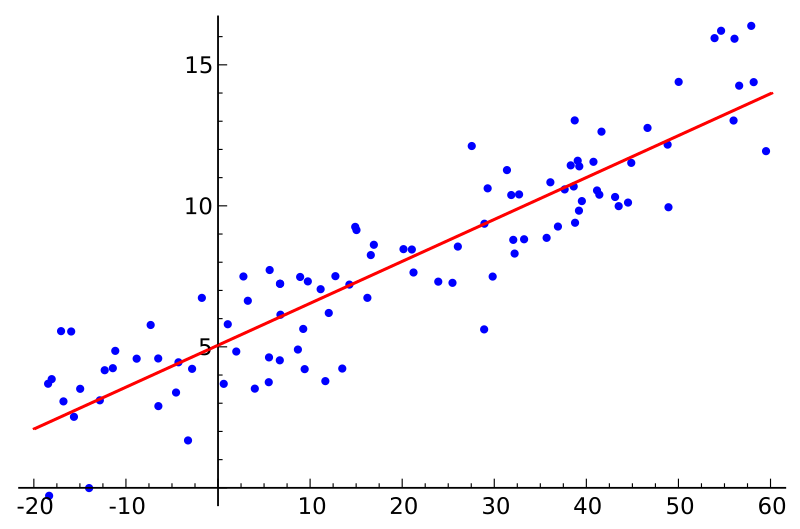
The blue dots are our $X$. The red line, a fitted simple linear regression, is our $Y$. For those familiar with regression, the $SSE$ (Sum of Squares of Errors, the shortest distance from our red line to each blue dot) would be our (reducible) $\epsilon$ in this particular case.
Motivation for Estimating $f$
So far, we’ve declared that there is a fixed and unknown function $f$ that, after inputting the values $X$ plus the error term $\epsilon$, can get us our output $Y$. But we don’t know $f$, so how can we use this equation?
The trick is to create an estimation of what $f$ should be.
In general, there are two things that we want from data: to predict and/or to infer. You can learn more about prediction and inference at the Prediction vs. Inference Starter Guide page. For our purposes, we are going to look at what estimating $f$ looks like in a prediction context.
Prediction
You will recall that a hat symbol (the ^ in $\hat{Y}$) represents the approximation, or estimation. So lets write out what the equation looks like with an estimation:
$ \hat{Y}=\hat{f}(X)$
This says: "The estimation of $Y$ is equivalent to the estimation of the function evaluated at $X$". We know what $X$ is; thats our data, which doesn’t need to be estimated because we’ve already collected it. In this case, the function $\hat{f}$ could be any function.
Reducibility of Error
But how accurate is $\hat{f}$ in estimating the actual $f$? Here, the error term $\epsilon$ is divvied up into two error terms, the so called reducible and irreducible error terms.
Reducible error is the error which we can improve by tweaking our analysis to better estimate $f$. The irreducible error is the error which is impossible to control for. It might come having noisy data, or a difficult modeling technique.
Mathematically, we can write this as
$E(Y-\hat{Y})^{2} =E[f(X)+\epsilon-\hat{f}(X)]^2$
$=\underbrace{[f(X)-\hat{f}(X)]^2}_{Reducible}+\underbrace{Var(\epsilon)}_{Irreducible}$
Where
$ E(Y-\hat{Y})^2 $
is the average/expected value ($E$ for expected) of the square difference between the estimated and actual value of $Y$, and
$ Var(\epsilon) $
is the variance of the error term, $\epsilon$.
The goal of data science in general is to minimize the reducible error so that we can approximate f well enough.
How Do We Estimate $f$?
While there are many techniques to model data, they can be broadly summarized into two distinct approaches: parametric and non-parametric.
Recall that our goal is find a function $\hat{f}$ that minimizes the reducible error enough that $Y\approx\hat{f}(X)$ for any observation $(X,Y)$.
Let’s see how this is done using the parametric approach.
Estimating $f$ Using The Parametric Approach
We are going to present a 2-step approach in the form of OLS (Ordinary Least Squares). There are many parametric approaches, but OLS is one of the most common and you might already have seen it used (if you’ve done any kind of regression then you’ve used OLS).
1. We make some basic assumption about the shape of $f$.
In OLS, we would start by modeling a linear equation that looks like
$ f(X) = \beta_0 + \beta_{1}x_1 + \beta_{2}x_2 + … + \beta_{p}x_p $
If you aren’t familiar with OLS, that’s ok; just know this is the standard form of an OLS equation.
You might recall that the $X$ values ($x_1, x_2, …, x_p$) are known, but what about the $\beta$ values? These are the parameters, also called coefficients, and these are what needs to be approximated to make our function work.
2. Now we fit, or train, the model.
Fitting entails using our training data to estimate the parameters.
In the case of OLS, finding the $\beta$ values means minimizing the $SSE$ (Sum of Squares of Errors); the procedure for doing this outside of the scope of this article, but once we have found the $\beta$ values which give the minimization of $SSE$ for the data $$, then we have our parameters.
Estimating $f$ Using The Non-Parametric Approach
In our previous example of OLS using the parametric approach, we had to assume that $f$ was approximately linear. But why did we make this assumption, without looking at the data? How did we know it wasn’t best approximated by a cubic equation?
The non-parametric approach avoids the question of assuming what kind of function $f$ might be. Instead, a function $f$ is chosen that matches the data points as closely as possible. One advantage of doing this is that the possibility of shapes of $f$ is near endless, and thus model fitting can be extremely flexible. However, a major disadvantage is that a large number of data observations is required to get an accurate approximation of $f$.
Refer to the image below for an example of a non-parametric technique, called splines.
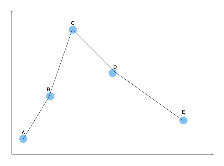
The above image is a spline fitted to 5 data points. You don’t need to know what a spline is, other than that it creates a line from point A to point B, point B to point C, etc. This makes it non-parametric; it merely creates a (typically) polynomial equation in a piecewise fashion (in this case, the black line which is our $\hat{f}(X)$ that goes through all the points).
To see the downsides of non-parametric approaches, imagine that we got one more random data point, marked by the green dot.
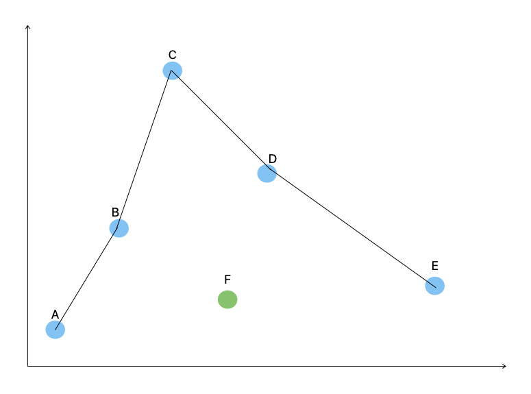
Our $\hat{f}(x)$ now doesn’t match our output $Y$ because the new data point (green dot) isn’t anywhere near our line! In some cases, we might say well, its close enough despite not being on the line. What degree of approximation, and thus prediction or inference, you need is entirely dependent on your problem.
This is an example of one of the disadvantages of non-parametric approaches: although they fit the data with a reducible error term of 0, when encountering new data they can be fairly off when trained on small amounts of data. In our example of 5+1 data points, we have very little data and a relatively simple polynomial equation to represent it. But what if we had millions of data points in $X$? We would have an incredibly complicated function that in theory would get a distribution of data points that represents what the data is typically like, and thus our non-parametric approach might be able to get a fairly good approximation. But all this hinges on having enough data.
Our Sources
-
www.statlearning.com, chapter 2.1.1