Curse of Dimensionality
Introduction
The Curse of Dimensionality refers to the difficulties in modeling high dimensional data. The word dimension is used in many different contexts with conflicting meanings, and even in the machine learning realm there are conflicting meanings. Here is a list from Google in the different ways the term dimension gets used:
-
The number of levels of coordinates in a Tensor. For example: A scalar has zero dimensions, such as ["Hello"]; a vector has one dimension, like [3, 5, 7, 11]; and a matrix has two dimensions, such as [[2, 4, 18], [5, 7, 14]]. You can uniquely specify a particular cell in a one-dimensional vector with one coordinate; you need two coordinates to uniquely specify a particular cell in a two-dimensional matrix.
-
The number of entries in a feature vector.
-
The number of elements in an embedding layer.
Dimensions, in the context of Curse of Dimensionality, really means entries in a feature vector (or variables; sometimes also called the feature space), and as such the Curse of Dimensionality refers to having too low a number of observations per dimension/feature; the confusion in terminology is unfortunate but "dimension" is one of those words, like "normal" or "standard" which gets thrown around a lot with different meanings in the sciences. For our purposes, we will use the word "feature" to mean the entries in the feature vector. We will reserve the word "dimension" for its usage as a "number of levels of coordinates in a tensor". This will make sense when you do the Power of PCA code example that you can find at the bottom of the page. Feature here would be the same as columns or variables, the things we are measuring.
Thus, the Curse of Dimensionality is having too few samples $n$ per feature $p$. As an example, having $n=3$ observations (or data points) and $p=500$ variables would lead to $\frac{3}{500}$ observations per feature. Imagine trying to train on this data. How would your model learn about these features if it only had 3 observations (and, realistically, at most 3 features for which it has any data at all on)? If we are trying to understand what these features mean, how can we discover that if we have so few observation points on each feature?
In the past, CoD often wasn’t a problem, because we typically had very few features and many observations. Think of something simple, like a questionnaire about health. Since mostly everything was handwritten, they might only have 10-15 questions, like age, sex, height, weight, etc. Then they hand this questionnaire out to 10,000 people. 10,0000 people (or observations/samples) divided by 10 features would be 1,000 observations/samples per feature, making it relatively easy to draw conclusions on the features and their relationships because we have so many observations per feature.
The Sparsity Connection
Sometimes, you will see the Curse of Dimensionality mentioned as being the result of having "sparse" data. Sparsity comes from linear algebra, and can be represented by matrices with many zeroes, such as this one:
\begin{pmatrix} 0 & 0 & 0 & 0 & 4 \\ 0 & 0 & 2 & 0 & 0 \\ 0 & 0 & 0 & 0 & 0 \\ 3 & 0 & 0 & 0 & 11 \\ 0 & 0 & 0 & 0 & 0 \\ \end{pmatrix}
| Although sparsity refers to many zeroes or ones in matrices, in data science, the curse of dimensionality refers to $p$ being far larger than $n$. They are similar concepts, with the difference being that in data science, we can’t say anything about the missing data, whereas in linear algebra they are set to be 0. The difference between 0 and the lack of data is important. |
Hughes/Peaking Phenomenon
The Peaking Phenomenon, or Hughes Phenomenon, has been known since the late 1960’s. It essentially states that there is an optimal size $n$ for any set of $p$ that minimizes the probability of training error.
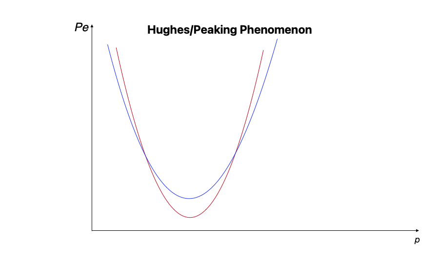
The blue line might be one set of $N=n_1$, and the red line would be a different set of observations where $N=n_2$. The goal is to choose the ideal $n$ and $p$ (labeled on the x axis) for your given problem to minimize the probability of training error ($P_e$ above).
You can learn more about the importance of choosing the optimal $n$ given any $p$ from Pattern Recognition (2009, Koutroumbas & Theodoridis). If you are interested in learning the research roots (and why its called the Hughes Phenomenon), check out On the Mean Accuracy of Statistical Pattern Recognizers (1968, Hughes).
How Can We Deal With The Curse of Dimensionality In Data Science?
Start By Calculating Your Features
To calculate the number of features, calculate the total columns/variables/features in the feature vector. It’s important to count them even if they are null or have no/missing data; the key word here is possible. Let’s look at an example of where we sample 10,000 color images with pixel features (2000,3000) and with standard RGB colors (3 total, Red Green and Blue; by default between 0 and 255).
$\underbrace{2000*3000}_{x*y}*\underbrace{3}_{RGB}=18,000,000$
| Image data is sometimes represented as 2, 3, or 4 dimensional data; this isn’t wrong per se, they just are operating with a different meaning of "dimension" that means something more along the lines of "the number of coordinates needed to specify a point". |
For image data, to create each pixel, we would have to select an x, y, R(ed), G(reen), and B(lue) value. For image data, each separate pixel value is its own feature. In our data, we have a sample size of $n=10,000$, meaning that we have $\frac{10,000}{18,000,000}=~.00056$ samples per feature.
But what does this samples per feature value really mean, and why does it matter? Imagine we are trying to learn about images of cats. If we only have 1 picture of a cat that is (2000,3000) and a color (so RGB color channel) image, then we’d only have 1 observation per each feature, because $n=1$! How are we going to learn about what a cat typically looks like in an image if we have so few training samples to go off? This is the crux of the Curse.
Consider another example, where we have a questionnaire with 50 variable responses, that is 50 features. We hand out our questionnaire to 50,000 people, and get a sample size of $n=50,000$. In this case, we would have 1,000 samples per feature. We’d certainly have much more to learn about each given feature!
The Obvious: Remove Features
If in our questionnaire example above, say only 4 of the feature are able to be answered, then maybe sticking to just those 4 is best, and removing the 46 others. Simple, but sometimes this doesn’t work: for instance, what if we discover that although people answer on average 4 features, they typically don’t answer the same 4? We would still have very sparse data. While this is an obvious approach, it almost never is useful because often our problem involves picking which features matter; this is a process called feature selection, or feature engineering. Wholesale removal of features is almost always a bad start because you typically aren’t sure of which features will be valuable until after you’ve done EDA or even the model training itself.
Dimensionality Reduction
Dimensionality reduction is a technique where we reduce the number of features while at the same time try to preserve the statistical signal embedded at each dimension. It is somewhat lossy, in that the statistical signal is not guaranteed to be preserved; however, dimensionality reduction techniques have proven incredibly useful as of late. Here is a list of some of the most common techniques in data science:
-
Principal Component Analysis (PCA) (see the coding example at the bottom of the page!)
-
Kernel PCA
-
Linear Discriminant Analysis (LDA)
-
Autoencoders
-
t-Distributed Stochastic Neighbor Embedding
-
Uniform Manifold Approximation and Projection (UMAP)
-
Generalized Discriminant Analysis (GDA)
$L_1$ Regularization
$L_1$ regularization is a technique where models are penalized via $|weight|$, where the absolute value of each individual weight in the model should be as small as possible. The Google article listed uses dimension to mean features, but the idea is the same: encourage models where there are as many zeroes as possible, which will create more computationally efficient models. This approach is great when you are having computational issues (that is, storing all your features and/or performing calculations in RAM).
Thinking About Your Problem
Sometimes, our data can present ways in which we can trim out features if we think carefully about the problem. An example of this can be found in analyzing healthcare x-ray images. We are given a set of a few hundred thousand x-rays of human skulls. We are tasked with identifying anomalies in the skulls. Given that our pixel (x,y) feature space is 2000*3000, our total features are
$\underbrace{2000*3000}_{x*y}*\underbrace{3}_{RGB}=18,000,000$
Above, the x*y are the pixel features of the image. The RGB is the Red, Green and Blue colors at each pixel (between 0 and 255).
Maybe, after EDA, we discover that the vast majority of the space around the edges is black; we notice that, if we just slice out 25% from the centered x and y values, we should be able to still capture all or mostly all of the skull but without all that black trim outline. So now our pixel features are 1500*2250.
It’s an x-ray image, so grayscale is what matters by nature of the x-ray. Somehow these are RGB; by converting RGB to grayscale, we would divide the features by 3 (because the 3 RGB color channels would go to 1 grayscale channel).
Now our total features would be:
$\underbrace{1500*2250}_{x*y}*\underbrace{1}_{Grayscale}=3,375,000$
Now, ~3 million features is still way too many- clearly other techniques are needed here, possibly autoencoding or PCA. But we reduced the total features almost by a factor of ~100, without doing much!
Thinking about the number of features in your problem, where they come from, and seeing if there are simple things you can do to reduce the features often is a great step.
Code Examples
| All of the code examples are written in Python, unless otherwise noted. |
Containers
| These are code examples in the form of Jupyter notebooks running in a container that come with all the data, libraries, and code you’ll need to run it. Click here to learn why you should be using containers, along with how to do so. |
| Quickstart: Download Docker, then run the commands below in a terminal. |
Power of PCA notebook
Power of PCA explores the basics of how PCA functions by finding the principal components in a single image as a demonstration and reconstructs the image from those principal components.
#pull container, only needs to be run once
docker pull ghcr.io/thedatamine/starter-guides:power-of-pca

#run container
docker run -p 8888:8888 -it ghcr.io/thedatamine/starter-guides:power-of-pca
Need help implementing any of this code? Feel free to reach out to [email protected] and we can help!