Geospatial Analytics using Python and SQL
Map Matching
Introduction to Map Matching
Sometimes GPS data are not as accurate as we would like:
-
Low sampling rate
-
Noise
-
Lack of granularity (i.e., number of decimal places in coordinate value)
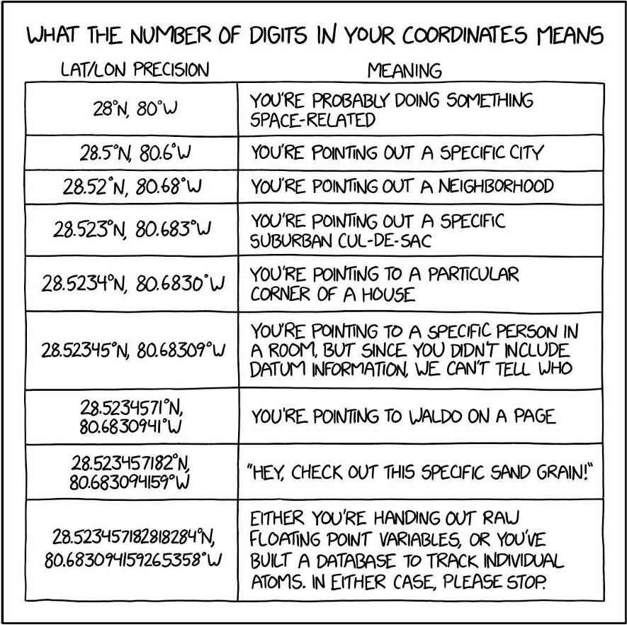
Without preprocessing and cleaning GPS data, small issues can concatenate into large, quality issues for our spatial analyses and maps. Take, for example, the map below. Do you see any issues with the placed GPS points?
When determining if the above map has issues to be addressed, please answer the following questions:
-
Are GPS points clearly on the road network?
-
Do GPS points stay on a single road/accurately depict where someone was driving?
Are GPS points clearly on the road network?
Remember, you can think of a road network as a graph—with many nodes connected by many edges. For many spatial analyses, graph theory and network analysis techniques are used, so it is imperative all points are reflected on the graph. Unfortunately, in our case, GPS data are very dirty here—spilling off our road network, either into buildings and the median, as well as on other roads. Without handling these issues, our analyses/maps generated from these data will be ambiguous and unreliable.
Do GPS points stay on a single road/accurately depict where someone was driving?
As with the above answer, no. GPS data are very dirty here—spilling off our road network, either into buildings and the median, as well as on other roads. With these data, we enter a great deal of ambiguity w.r.t. driver location and behavior on the road network.
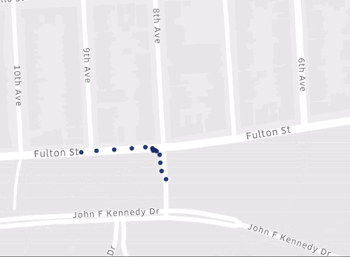
This is where map matching comes in!
From the human eye, we can confidently determine that our driver was driving on the road, and not taking a convoluted path on and off a busy road, but the computer and models do not know this, which will cause problems when doing analyses. Thus, we must project (i.e., predict) where dirty GPS points belong on our map.
To do these projects, we employ a technique called map matching: "taking raw GPS data and a respective road network as input, and giving output as the actual position of aforementioned GPS points on the provided road network." An example of this projection is depicted below:
Why is Map Matching Important?
Let’s look at a ride-hailing example (e.g., Uber). When generating routes, Uber wants to minimize the distance and time to reach a destination:
-
Distance: Decreased wear on drivers’ vehicles and reduction in fuel required to execute a trip.
-
Time: A driver can accomplish more rides in a shift and the customer gets to their destination faster.
There are two map matching approaches covered in this section:
-
Via Hidden Markov Models (i.e., home-grown)
-
Via Python (i.e., out-of-the-box implementation)
Review of Markov Chains
Before we can understand hidden markov models, let alone map matching, we should first touch on markov chains. A Markov chain is a stochastic model describing a sequence of possible events in which the probability of each event depends only on the state attained in the previous event. But, what does this look like in practice?
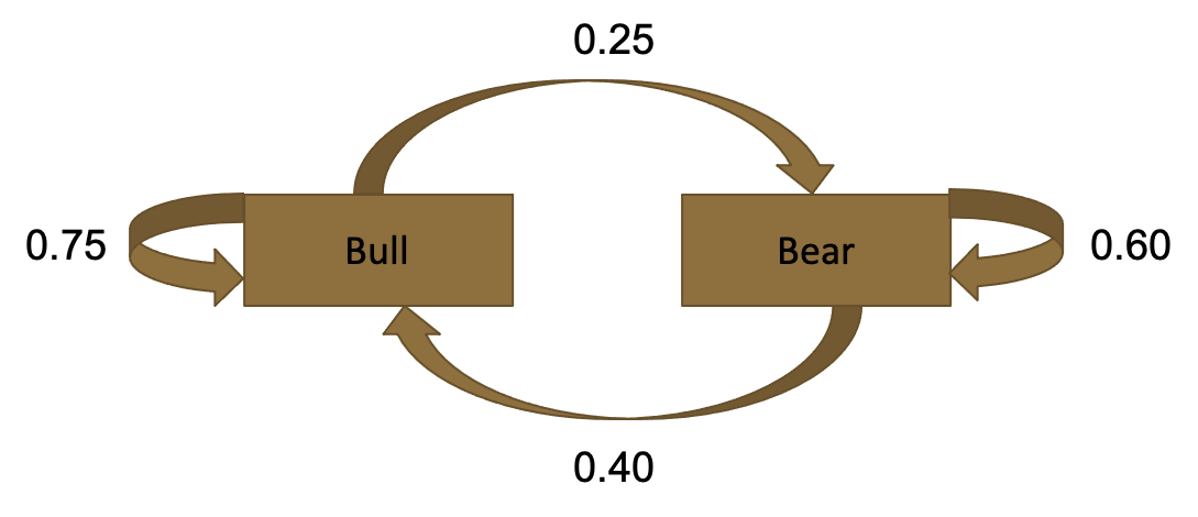
We will use an example from the stock market. The question we are trying to answer is, given the following market information, if we have a bull market this week, what are the probabilities of a bull vs. bear market in teo weeks?
Information:
-
75% a bull market followed by a bull market (going up)
-
60% a bear market followed by a bear market (going down)
First, let’s start by setting up the problem. In our scenario, the market can be in either one of two states: bear or bull.
We have information w.r.t. probable market movement in following weeks, based on the current week’s market state. With this information, we can set up the following diagram:
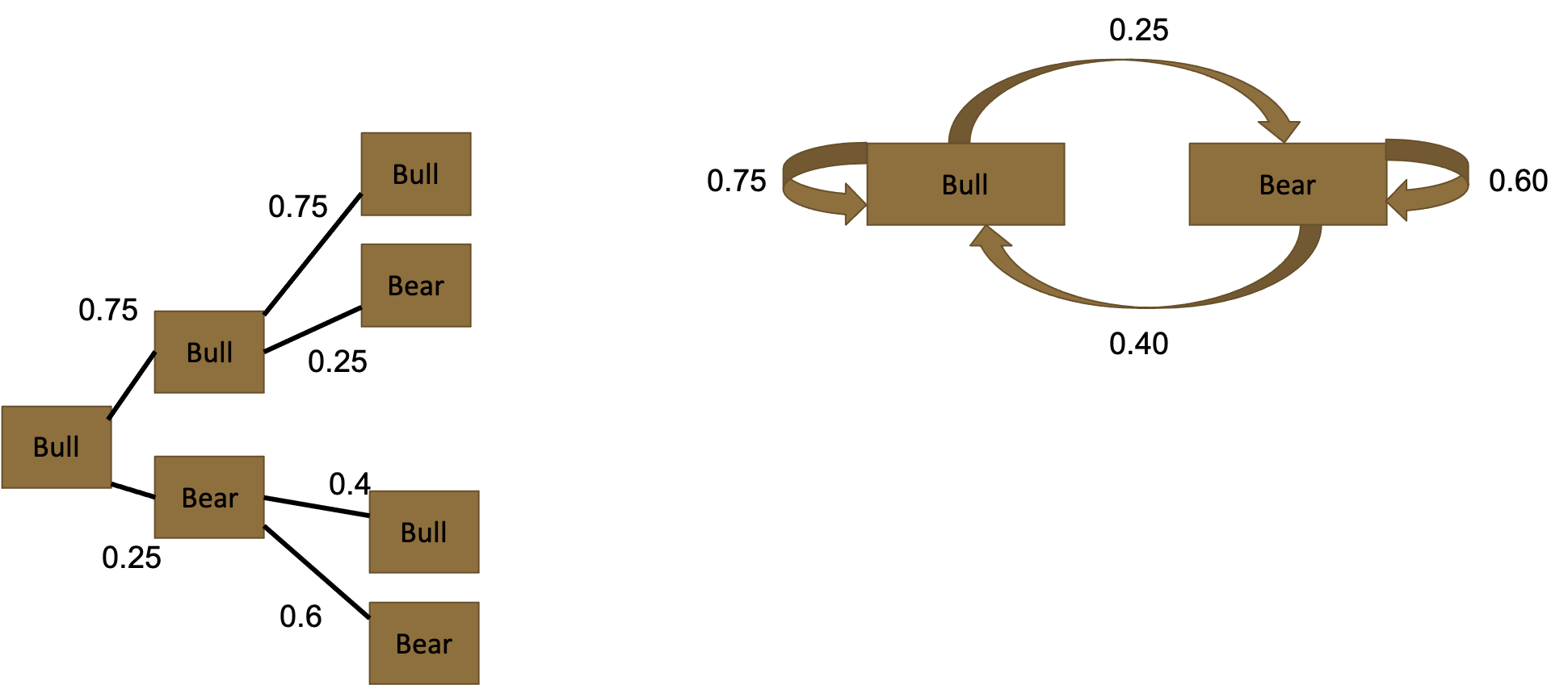
We are looking for market state in two weeks, given that this week is a bull market. Therefore, we set up a tree starting at a bull market, and simulating market states for two cycles (i.e., weeks in this example). This gives us the following tree on the left:
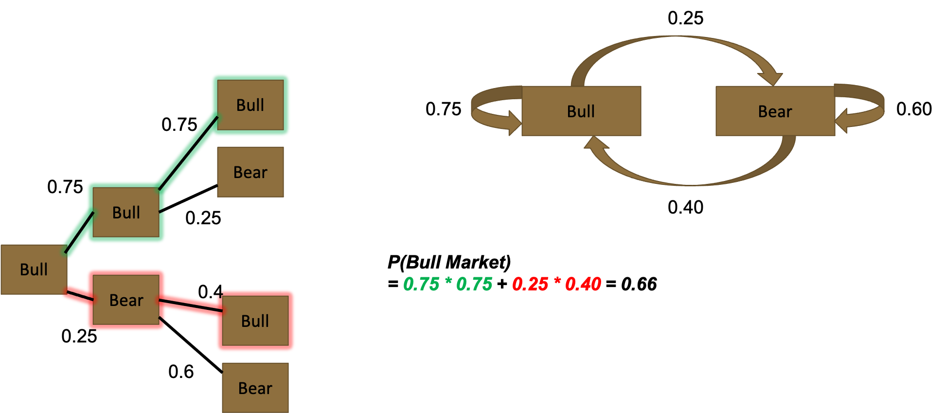
We can now predict probability of a bull market in two weeks, by following the green and red highlighting:

Hidden Markov Models for Map Matching
Let’s use HMMs for map matching. This is the approach Uber takes for its map matching. Let’s visualize and explain the problem.
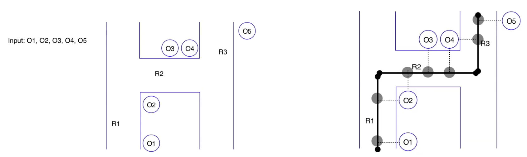
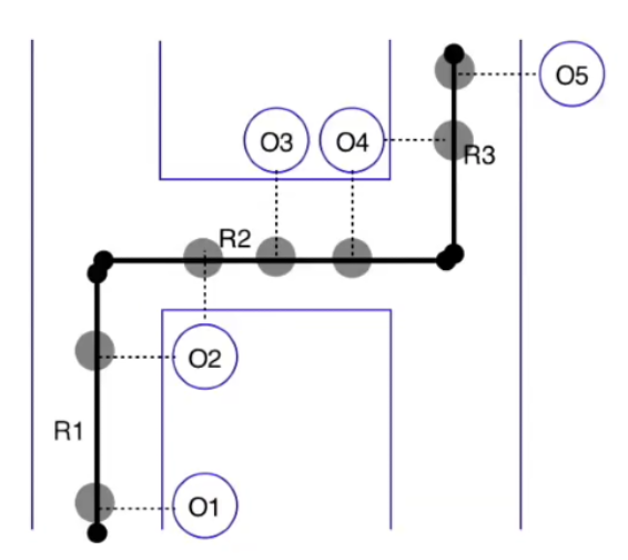
In essence, we have GPS points (O) and a given road network with road segments (R). We are trying to go from ambiguous GPS data on the left, to an inferred route, as depicted on the right. Thus, we are attempting to predict the probability of a GPS point belonging to a specific road segment at a certain point in time, in sequence of the driver’s route.
Let’s further set up our problem.
-
R1-R3= road segments -
O1-O5= GPS observations
Our goal is to figure out for every GPS observation, which road segment, in theory, could have produced that GPS point.
To do this, candidate road segments are generated via kNN lookup (i.e., look up k closest road segments within search radius). Once candidate segments are identified, draw the projection of that GPS signal on road signal, which is a line perpendicular from signal to candidate road segment.
These projections are depicted as the transparent circles in the image on the right. Note that observations can have multiple segment candidates (e.g., O2 and O4 can be projected to R1/R2 or R2/R3, respectively).
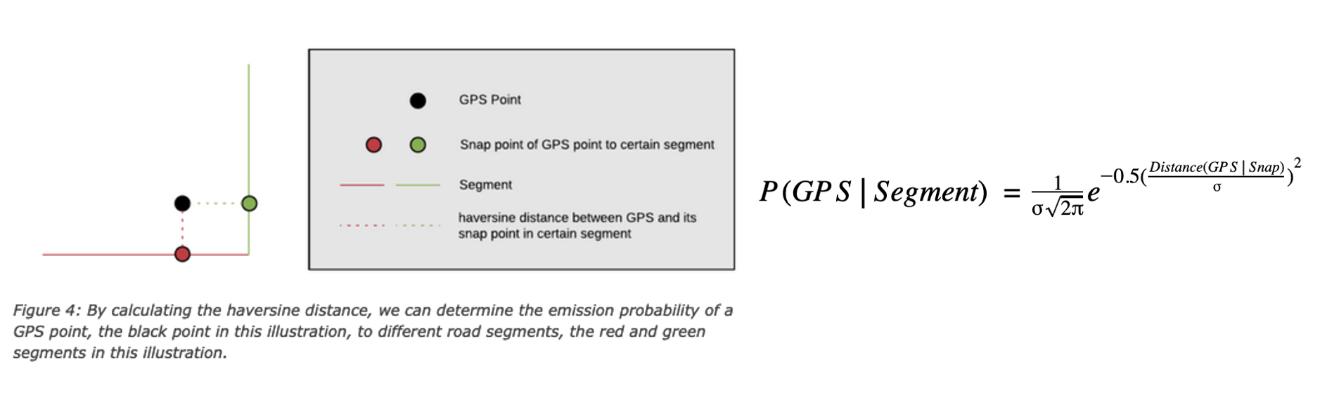
The emission probability represents the likelihood of a vehicle present on certain road segments at certain moments.
For example, let’s take R3 and O5. We are trying to calculate the probability of seeing O5 if the car was traversing on R3. This is to be calculated by function of great circle distance between GPS signal and its projection for a given candidate road segment.
-
Great Circle Distance (i.e., Haversine distance): The shortest path between 2 points on Earth (following allowing the curvature of the earth). Tis DOES NOT follow topology of road network.
-
Shortest Path Distance: Follows topology of road network (graph), while accounting for the rules of the road (e.g., one-way streets, legal turns, etc.) and traverse across legal edges
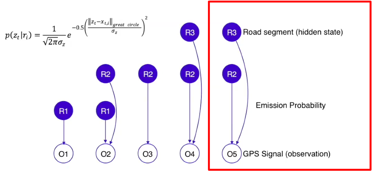
For one GPS point with m number of road segments nearby, there will be m emission probabilities representing the likelihood of this GPS trace on each road segment.
For GPS points G1, which have m nearby segments, and G2, which has n nearby segments, there are m * n transition probabilities. These probabilities are in HMM, in which they pick up a sequence of states with maximum probabilities that are most likely to represent road segments on which the vehicle was moving.
The haversine distance between the GPS point and its snap point on the road segment. The emission probability indicates how likely the GPS would be observed if the vehicle is actually on the road segment.
We then calculating transition probability regarding one GPS point on a certain segment to another GPS point on a certain segment, calculated using the following formula. This formula is called DistanceDiff, and is defined as the following: the absolute value of the difference between the haversine distance of two GPS points and the routable distance between two snap points associated with the GPS points.
It is less likely that the vehicle was traversing through these two segments when emitting GPS positions if DistanceDiff is greater than others.
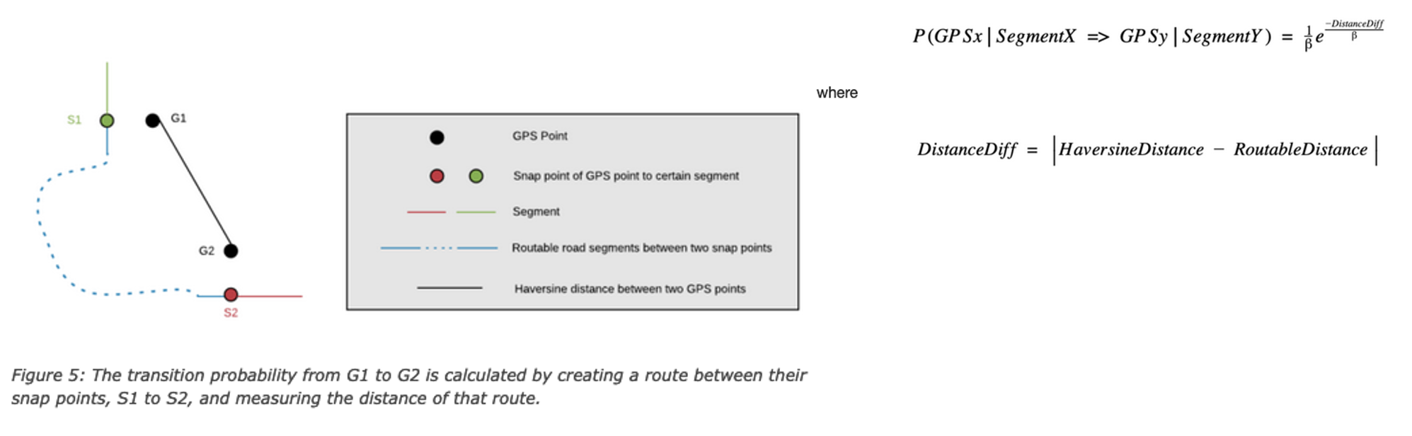
Now, we have to look at the transition probability of our HMM. In this example, the transition probability represents the likelihood of a vehicle moving from one road segment to another road segment over a certain duration.
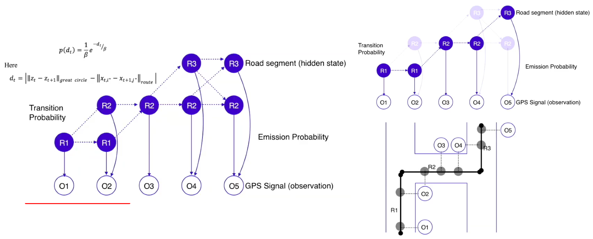
An example transition probability to calculate is for R1, R2 – the probability the car traversed from R1 to R2.
An assumption we can make is that certain road transitions should be more likely than others. Any transition that provides a feasible route has a higher transition probability. A feasible route is the difference between the haversine distance and the shortest path distance between the two projections is closest to 0.
By calculating the transition probability, we can show the driver’s trip unfolding, following where they traversed. This concludes with the following trip recorded for our driver:
Python for Map Matching
We will be working through the tutorials within leuvenmapmatching’s
documentation:
leuvenmapmatching.readthedocs.io/en/latest/index.html
Required Packages
*In[54]:*
#General
import leuvenmapmatching
import osmread
from pathlib import Path
import requests
import rtree
import pyproj
#Visualization from leuvenmapmatching import visualization as mmviz
#Examples from leuvenmapmatching.matcher.distance import DistanceMatcher from leuvenmapmatching.map.inmem import InMemMap from leuvenmapmatching.util.gpx import gpx_to_path
Example 1: Simple
leuvenmapmatching.readthedocs.io/en/latest/usage/introduction.html#example-1-simple
A first, simple example. Some parameters are given to tune the
algorithm. The max_dist and obs_noise are distances that indicate
the maximal distance between observation and road segment and the
expected noise in the measurements, respectively. The min_prob_norm
prunes the lattice in that it drops paths that drop below 0.5 normalized
probability. The probability is normalized to allow for easier reasoning
about the probability of a path. It is computed as the exponential
smoothed log probability components instead of the sum as would be the
case for log likelihood.
*In[3]:*
#Define an Arbitrary Map
map_con = InMemMap("mymap", graph={
    "A": ((1, 1), ["B", "C", "X"]),
    "B": ((1, 3), ["A", "C", "D", "K"]),
    "C": ((2, 2), ["A", "B", "D", "E", "X", "Y"]),
    "D": ((2, 4), ["B", "C", "F", "E", "K", "L"]),
    "E": ((3, 3), ["C", "D", "F", "Y"]),
    "F": ((3, 5), ["D", "E", "L"]),
    "X": ((2, 0), ["A", "C", "Y"]),
    "Y": ((3, 1), ["X", "C", "E"]),
    "K": ((1, 5), ["B", "D", "L"]),
    "L": ((2, 6), ["K", "D", "F"])
}, use_latlon=False)
#Define GPS Points to Map Match path = [(0.8, 0.7), (0.9, 0.7), (1.1, 1.0), (1.2, 1.5), (1.2, 1.6), (1.1, 2.0), (1.1, 2.3), (1.3, 2.9), (1.2, 3.1), (1.5, 3.2), (1.8, 3.5), (2.0, 3.7), (2.3, 3.5), (2.4, 3.2), (2.6, 3.1), (2.9, 3.1), (3.0, 3.2), (3.1, 3.8), (3.0, 4.0), (3.1, 4.3), (3.1, 4.6), (3.0, 4.9)]
matcher = DistanceMatcher(map_con, max_dist=2, obs_noise=1, min_prob_norm=0.5) states, _ = matcher.match(path) nodes = matcher.path_pred_onlynodes
print("States\n--") print(states) print("Nodes\n--") print(nodes) print("") matcher.print_lattice_stats()
*Out[3]:*
/Users/gould29/opt/anaconda3/envs/honr490/lib/python3.7/site-packages/pyproj/crs/crs.py:53: FutureWarning: '+init=<authority>:<code>' syntax is deprecated. '<authority>:<code>' is the preferred initialization method. When making the change, be mindful of axis order changes: https://pyproj4.github.io/pyproj/stable/gotchas.html#axis-order-changes-in-proj-6
  return _prepare_from_string(" ".join(pjargs))
Searching closeby nodes with linear search, use an index and set max_dist
States
[('X', 'A'), ('A', 'B'), ('A', 'B'), ('A', 'B'), ('A', 'B'), ('A', 'B'), ('A', 'B'), ('A', 'B'), ('B', 'D'), ('B', 'D'), ('B', 'D'), ('B', 'D'), ('D', 'E'), ('D', 'E'), ('D', 'E'), ('E', 'F'), ('E', 'F'), ('E', 'F'), ('E', 'F'), ('E', 'F'), ('E', 'F'), ('E', 'F')] Nodes
Stats lattice - nbr levels : 22 nbr lattice : 1002 avg lattice[level] : 45.54545454545455 min lattice[level] : 7 max lattice[level] : 97 avg obs distance : 0.15514927458475236 last logprob : -0.5464565099511667 last length : 22 last norm logprob : -0.024838932270507576
Now, we will visualize the above map, via leuvenmapmatching.readthedocs.io/en/latest/usage/visualisation.html
*In[7]:*
mmviz.plot_map(map_con, matcher=matcher,
               show_labels=True, show_matching=True, show_graph=True,
               filename="example_1_plot.png")
*Out[7]:* (None, None)
The file should look like:
Let’s try visualizing an overlay of OpenStreetMaps:
*In[12]:*
mmviz.plot_map(map_con, matcher=matcher,
                use_osm=True, zoom_path=True,
                show_labels=False, show_matching=True, show_graph=False,
                filename="example_1_osm_plot.png")
*Out[12]:*
Lowered zoom level to keep map size reasonable. (z = 7)
(None, <matplotlib.axes._subplots.AxesSubplot at 0x7fb09be5dc50>)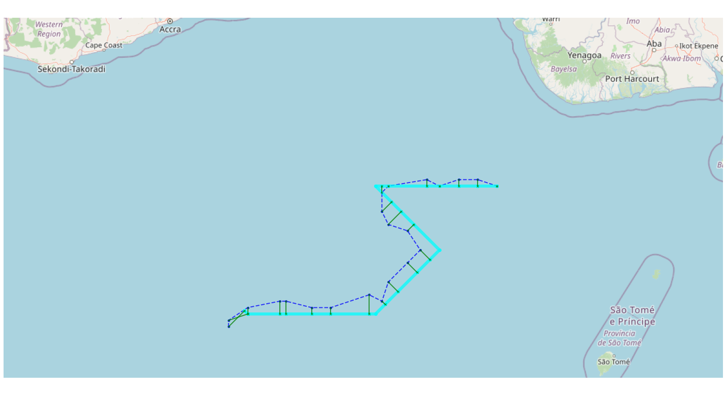
Example 2: Non-emitting States
leuvenmapmatching.readthedocs.io/en/latest/usage/introduction.html#example-2-non-emitting-states
In case there are less observations that states (an assumption of HMMs),
non-emittings states allow you to deal with this. States will be
inserted that are not associated with any of the given observations if
this improves the probability of the path.
It is possible to also associate a distribtion over the distance between
observations and the non-emitting states (obs_noise_ne). This allows
the algorithm to prefer nearby road segments. This value should be
larger than obs_noise as it is mapped to the line between the previous
and next observation, which does not necessarily run over the relevant
segment. Setting this to infinity is the same as using pure non-emitting
states that ignore observations completely.
*In[14]:*
#Define Points to Map Match
path = [(1, 0), (7.5, 0.65), (10.1, 1.9)]
#Define a Map to which Points are Mapped mapdb = InMemMap("mymap", graph={ "A": ((1, 0.00), ["B"]), "B": ((3, 0.00), ["A", "C"]), "C": ((4, 0.70), ["B", "D"]), "D": ((5, 1.00), ["C", "E"]), "E": ((6, 1.00), ["D", "F"]), "F": ((7, 0.70), ["E", "G"]), "G": ((8, 0.00), ["F", "H"]), "H": ((10, 0.0), ["G", "I"]), "I": ((10, 2.0), ["H"]) }, use_latlon=False)
matcher = DistanceMatcher(mapdb, max_dist_init=0.2, obs_noise=1, obs_noise_ne=10, non_emitting_states=True, only_edges=True) states, _ = matcher.match(path) nodes = matcher.path_pred_onlynodes
print("States\n--") print(states) print("Nodes\n--") print(nodes) print("") matcher.print_lattice_stats()
mmviz.plot_map(mapdb, matcher=matcher, show_labels=True, show_matching=True, filename="example_2_plot.png")
*Out[14]:*
/Users/gould29/opt/anaconda3/envs/honr490/lib/python3.7/site-packages/pyproj/crs/crs.py:53: FutureWarning: '+init=<authority>:<code>' syntax is deprecated. '<authority>:<code>' is the preferred initialization method. When making the change, be mindful of axis order changes: https://pyproj4.github.io/pyproj/stable/gotchas.html#axis-order-changes-in-proj-6
  return _prepare_from_string(" ".join(pjargs))
Searching closeby nodes with linear search, use an index and set max_dist
States
[('A', 'B'), ('B', 'C'), ('C', 'D'), ('D', 'E'), ('E', 'F'), ('F', 'G'), ('G', 'H'), ('H', 'I')] Nodes
Stats lattice - nbr levels : 3 nbr lattice : 40 avg lattice[level] : 13.333333333333334 min lattice[level] : 8 max lattice[level] : 16 avg obs distance : 0.26790850746762634 last logprob : -2.373678241605297 last length : 3 last norm logprob : -0.791226080535099 (None, None)
Using OSM and Applying a Sample GPS Trace Trip (Walking): Detroit, MI
leuvenmapmatching.readthedocs.io/en/latest/usage/openstreetmap.html
The next section requires OSM data. OSM is open source maps and map
data. Free!
Download a Sample Map
*In[37]:*
xml_file = Path(".") / "sample_osm.xml"
url = 'http://overpass-api.de/api/map?bbox=-83.0680102,42.3510973,-82.9575603,42.357894'
r = requests.get(url, stream=True)
with xml_file.open('wb') as ofile:
    for chunk in r.iter_content(chunk_size=1024):
        if chunk:
            ofile.write(chunk)
Create Graph
Once we have a file containing the region we are interested in, we can select the roads we want to use to create a graph from. In this case we focus on `ways' with a `highway' tag. Those represent a variety of roads. For a more detailed filtering look at the possible values of the highway tag.
*In[48]:*
#Create Map Connection via OSM
map_con = InMemMap("myosm", use_latlon=True, use_rtree=False, index_edges=True)
for entity in osmread.parse_file(str(xml_file)): if isinstance(entity, osmread.Way) and 'highway' in entity.tags: for node_a, node_b in zip(entity.nodes, entity.nodes[1:]): map_con.add_edge(node_a, node_b) # Some roads are one-way. We’ll add both directions. map_con.add_edge(node_b, node_a) if isinstance(entity, osmread.Node): map_con.add_node(entity.id, (entity.lat, entity.lon)) map_con.purge()
*Out[48]:*
/Users/gould29/opt/anaconda3/envs/honr490/lib/python3.7/site-packages/pyproj/crs/crs.py:53: FutureWarning: '+init=<authority>:<code>' syntax is deprecated. '<authority>:<code>' is the preferred initialization method. When making the change, be mindful of axis order changes: https://pyproj4.github.io/pyproj/stable/gotchas.html#axis-order-changes-in-proj-6
  return _prepare_from_string(" ".join(pjargs))
Map Match from OSM
*In[49]:*
%%time
#Read Traces
track = gpx_to_path("mytrack.gpx")
#Remove Extra None from track
track = [(lambda x: x[0:2])(x) for x in track]
matcher = DistanceMatcher(map_con, max_dist=100, max_dist_init=25, # meter min_prob_norm=0.001, non_emitting_length_factor=0.75, obs_noise=50, obs_noise_ne=75, # meter dist_noise=50, # meter non_emitting_states=True) states, lastidx = matcher.match(track)
*Out[49]:*
Searching closeby nodes with linear search, use an index and set max_distCPU times: user 2min 10s, sys: 1.61 s, total: 2min 12s Wall time: 2min 35s
*In[74]:*
track*Out[74]:*
[(42.355618, -83.054237),
 (42.35562, -83.054238),
 (42.355615, -83.054253),
 (42.355684, -83.054297),
 (42.355719, -83.054198),
 (42.355781, -83.054022),
 (42.355749, -83.054001),
 (42.355781, -83.054022),
 (42.355719, -83.054198),
 (42.35565, -83.054155),
 (42.355587, -83.054116),
 (42.355656, -83.053914),
 (42.35573, -83.053715),
 (42.355749, -83.053728),
 (42.35573, -83.053715),
 (42.355656, -83.053914),
 (42.355722, -83.05396),
 (42.355839, -83.053635),
 (42.355918, -83.053637),
 (42.355993, -83.053428),
 (42.355967, -83.053411),
 (42.355993, -83.053428),
 (42.355918, -83.053637),
 (42.355839, -83.053635),
 (42.355886, -83.053504),
 (42.355999, -83.053194),
 (42.356038, -83.053086),
 (42.356027, -83.053079),
 (42.356038, -83.053086),
 (42.356105, -83.052904),
 (42.356126, -83.052918),
 (42.356105, -83.052904),
 (42.355999, -83.053194),
 (42.355933, -83.053149),
 (42.35602, -83.052916),
 (42.35609, -83.052727),
 (42.356102, -83.052735),
 (42.35609, -83.052727),
 (42.35602, -83.052916),
 (42.355933, -83.053149),
 (42.355999, -83.053194),
 (42.356243, -83.052523),
 (42.356265, -83.052537),
 (42.356243, -83.052523),
 (42.3563, -83.052367),
 (42.356273, -83.052349),
 (42.3563, -83.052367),
 (42.356362, -83.052196),
 (42.356388, -83.052125),
 (42.356409, -83.052139),
 (42.356407, -83.052145),
 (42.356409, -83.052139),
 (42.35646, -83.052173),
 (42.356499, -83.052073),
 (42.356424, -83.052024),
 (42.356348, -83.051973),
 (42.35638, -83.051886),
 (42.356395, -83.051847),
 (42.356423, -83.051866),
 (42.356395, -83.051847),
 (42.35638, -83.051886),
 (42.356348, -83.051973),
 (42.356424, -83.052024),
 (42.356457, -83.051932),
 (42.356562, -83.051641),
 (42.356578, -83.051652),
 (42.356562, -83.051641),
 (42.35672, -83.051204),
 (42.356732, -83.051212),
 (42.35672, -83.051204),
 (42.356722, -83.051198),
 (42.356795, -83.050995),
 (42.356827, -83.051015),
 (42.356816, -83.051046),
 (42.356827, -83.051015),
 (42.356795, -83.050995),
 (42.356724, -83.050952),
 (42.356761, -83.050841),
 (42.356838, -83.050876),
 (42.356865, -83.050894),
 (42.356859, -83.050911),
 (42.356865, -83.050894),
 (42.356838, -83.050876),
 (42.356923, -83.050643),
 (42.356891, -83.050622),
 (42.356923, -83.050643),
 (42.356999, -83.050433),
 (42.356927, -83.050386),
 (42.356953, -83.050315),
 (42.356978, -83.050332),
 (42.356953, -83.050315),
 (42.356927, -83.050386),
 (42.35684, -83.050328),
 (42.356827, -83.050364),
 (42.35684, -83.050328),
 (42.356722, -83.050249),
 (42.35674, -83.050198),
 (42.356722, -83.050249),
 (42.356506, -83.050105),
 (42.356494, -83.050139),
 (42.356506, -83.050105),
 (42.356443, -83.050063),
 (42.356431, -83.050096),
 (42.356443, -83.050063),
 (42.356388, -83.050025),
 (42.356399, -83.049994),
 (42.356388, -83.050025),
 (42.356357, -83.050005),
 (42.356345, -83.049897),
 (42.356349, -83.049884),
 (42.35638, -83.049903),
 (42.356349, -83.049884),
 (42.356386, -83.049777),
 (42.356407, -83.04979),
 (42.356386, -83.049777),
 (42.356464, -83.049549),
 (42.356459, -83.049533)]
Visualize Results
*In[51]:*
mmviz.plot_map(map_con, matcher=matcher,
                use_osm=True, zoom_path=True,
                show_labels=False, show_matching=True, show_graph=False,
                filename="example_3_osm_plot.png")
*Out[51]:*
Lowered zoom level to keep map size reasonable. (z = 17)
(None, <matplotlib.axes._subplots.AxesSubplot at 0x7fb0a2b7be10>)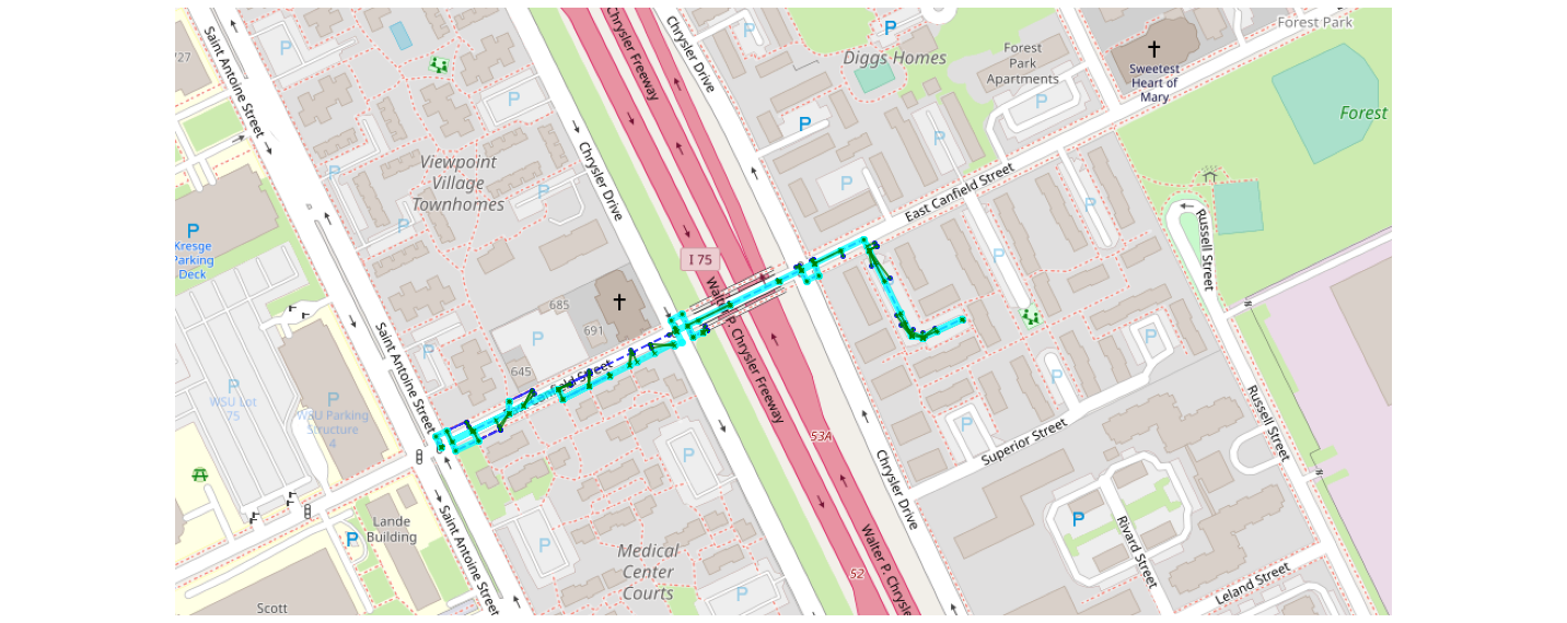
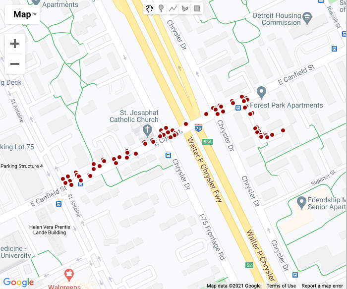
Look at the blue lines and green arrows to see projections made by the model. The light blue line represents the predicted path…points matched to our map. For reference, here is what the points look like just mapped out:
Apply to Latitude/Lognitude Data - (Back to the Documentation Demo!)
leuvenmapmatching.readthedocs.io/en/latest/usage/latitudelongitude.html
The toolbox can deal with latitude-longitude coordinates directly. Map
matching, however, requires a lot of repeated computations between
points and latitude-longitude computations will be more expensive than
Euclidean distances.
There are three different options how you can handle latitude-longitude coordinates: 1. Use Lat/Long Directly 2. Project Lat/Long to X/Y 3. Use Lat/Long as if they were X/Y
Option 1: Use Lat/Long Directly
leuvenmapmatching.readthedocs.io/en/latest/usage/latitudelongitude.html#option-1-use-latitude-longitude-directly
Set the use_latlon flag in the Map to true.
For example to read in an OpenStreetMap file directly to a InMemMap
object:
This is the same as above, so we will skip it
Option 2: Project Lat/Long to X/Y
Latitude-Longitude coordinates can be transformed two a frame with two orthogonal axis.
*In[52]:*
map_con_latlon = InMemMap("myosm", use_latlon=True)
# Add edges/nodes
map_con_xy = map_con_latlon.to_xy()
route_latlon = [] # Add GPS locations route_xy = [map_con_xy.latlon2yx(latlon) for latlon in route_latlon]
*Out[52]:*
/Users/gould29/opt/anaconda3/envs/honr490/lib/python3.7/site-packages/pyproj/crs/crs.py:53: FutureWarning: '+init=<authority>:<code>' syntax is deprecated. '<authority>:<code>' is the preferred initialization method. When making the change, be mindful of axis order changes: https://pyproj4.github.io/pyproj/stable/gotchas.html#axis-order-changes-in-proj-6
  return _prepare_from_string(" ".join(pjargs))
This can also be done directly using the pyproj toolbox. For example, using the Lambert Conformal projection to project the route GPS coordinates:
*In[66]:*
route = [(4.67878,50.864),(4.68054,50.86381),(4.68098,50.86332),(4.68129,50.86303),(4.6817,50.86284),
         (4.68277,50.86371),(4.68894,50.86895),(4.69344,50.86987),(4.69354,50.86992),(4.69427,50.87157),
         (4.69643,50.87315),(4.69768,50.87552),(4.6997,50.87828)]
lon_0, lat_0 = route[0]
proj = pyproj.Proj(f"+proj=merc +ellps=GRS80 +units=m +lon_0={lon_0} +lat_0={lat_0} +lat_ts={lat_0} +no_defs")
xs, ys = [], []
for lon, lat in route:
    x, y = proj(lon, lat)
    xs.append(x)
    ys.append(y)
#Create Set of GPS Points Converted to GRS80 to_map = [] for x, y in zip(xs, ys): to_map.appendx, y
to_map
*Out[66]:*
[(0.0, 4151393.067831352),
 (123.90874196328781, 4151371.931197072),
 (154.88592745410978, 4151317.4213293632),
 (176.71076268625436, 4151285.160658549),
 (205.57586734820242, 4151264.024466364),
 (280.9067502462715, 4151360.8066874975),
 (715.2913740607927, 4151943.763296859),
 (1032.1034983987597, 4152046.121256038),
 (1039.1437678284515, 4152051.684246792),
 (1090.537734665558, 4152235.266307333),
 (1242.60755434778, 4152411.0661618263),
 (1330.6109222194282, 4152674.7771780347),
 (1472.8243647000147, 4152981.9006716586)]
Option 3: Use Lat/Long as if they were X/Y
leuvenmapmatching.readthedocs.io/en/latest/usage/latitudelongitude.html#option-3-use-latitude-longitude-as-if-they-are-x-y-points
A naive solution would be to use latitude-longitude coordinate pairs as
if they are X-Y coordinates. For small distances, far away from the
poles and not crossing the dateline, this option might work. But it is
not advised.
For example, for long distances the error is quite large. In the image beneath, the blue line is the computation of the intersection using latitude-longitude while the red line is the intersection using Eucludean distances.

