Bias-Variance Tradeoff
Motivation
One of the most essential notions in modern data science is the bias-variance tradeoff. The general idea is that developing models always is a balance between models that vary too much, and models which are too heavily biased.
Developing Intuition
Let’s imagine the extremes of model building. You could in theory make a function that always equals some random number, say 5: $ f(x) = 5 $. So regardless of the values of x, we always return 5. This is an example of a model that is completely biased, and is one extreme of our bias variance tradeoff. Models that lean towards the bias extreme are experiencing what is called underfitting. When it comes to making predictions, this sort of model learns from the data less and less, hence its high error rate.
The other end is a model which varies so much that it doesn’t generalize well. This is called overfitting, and is when a model matches the data so closely that it fails to generalize to new data. An example of this might be a neural network model trained on images of cats. Imagine that, of our dataset of 50,000 cat images, almost all of them are cats that are outdoors. After training on these images, the net might pick up that the color green, or maybe even trees, are associated with cats. In this case, we might get a very high training accuracy, but after using a test set on images of cats that are indoors, we find our accuracy to be quite low- because our net thinks that cats should include green or trees in the image! This model has learned from the training data too well, and its predictions also cause high error rates.
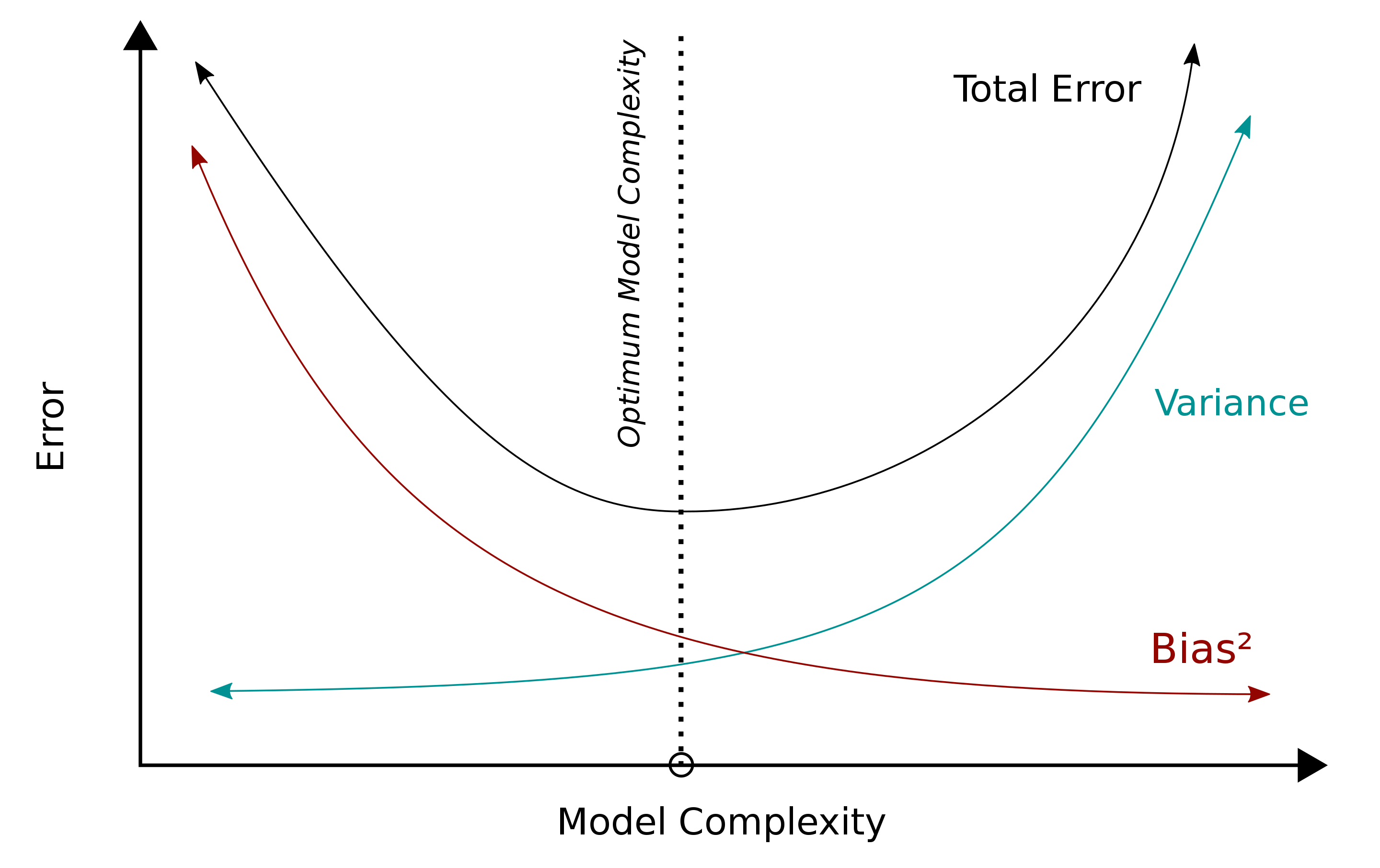
The basic idea behind bias-variance tradeoff is there is a sweetspot in the middle between these two extremes, and there are ways to mathematically show the approximate equilibrium and to minimize the error in predicting on the test set.
We can conclude with the Occam’s Razor of data science: models should never be more complex than they need to be.
A More Rigorous Definition
It is possible to show that the expected test MSE (Mean Squared Error) for a model, with a given input of $x_0$, can be decomposed into 3 quantities:
-
variance of $\hat{f}(x_0)$
-
squared bias of $\hat{f}(x_0)$
-
variance of the error term, $ \epsilon $.
Recall that $\hat{f}(x_0)$ means "the estimated value of function f given some value x". Mathematically, this can be written as
$ E(y_0 - \hat{f}(x_0))^2 = Var(\hat{f}(x_0)) + [Bias(\hat{f}(x_0))]^2 + Var(\epsilon) $
We can see the 3 quantities, but what does $ E(y_0 - \hat{f}(x_0))^2 $ mean? This is the "expected test MSE at $ x_0 $", which is our average test MSE that we’d get if we repeatedly estimated $ \hat{f} $ with many training sets, testing each time at $ x_0 $.
Commentary
One important thing to notice about this equation is that to minimize the expected test error, we need to get both a low variance, and low bias. However, both variance and bias (squared) are nonnegative. Even if we had an $ \epsilon $ of 0, our bias and variance would at best be equivalent to, but never lower than, our error rate. This is called the irreducibility of the error term. In practice, the error term is almost certainly going to be greater than 0; few models are perfect, and even when they are, they aren’t perfect for long.
The important thing to notice here is that we always going to have some noise in our signal; the noise is our $ \epsilon $.
Minimizing Bias/Dealing With Underfitting
-
Adding more features (can also lead to more variance)
-
Mixture models, ensemble learning
-
Increasing data
-
Fine tuning hyperparameters
Minimizing Variance/Dealing With Overfitting
-
Dimensionality reduction
-
Feature selection
-
Larger training set/increasing data
-
Data augmentation
-
Fine tuning hyperparameters