401 Project 08 - Classifiers - Decision Tree Ensembles
Project Objectives
In this project, we will be learning about Extra Trees and Random Forests, two popular ensemble models utilizing Decision Trees.
Questions
Question 1 (2 points)
In the last project, we learned about Decision Trees. As a brief recap, Decision Trees are a type of model that classify data based on a series of conditions. These conditions are found during training, where the model will attempt to split the data into groups that are as pure as possible (100% pure being a group of datapoints that only contains a single class). As you may remember, one fatal downside of Decision Trees is how prone they are to overfitting.
Extra Trees and Random Forests help address this downside by creating an ensemble of multiple decision trees.
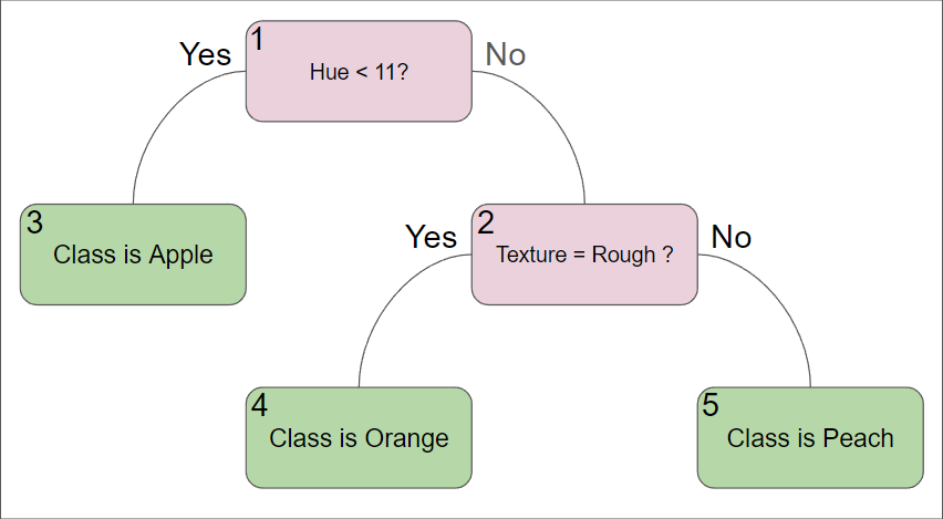
To review how a decision tree works, please classify the following three data points using the below decision tree.
| Hue | Weight | Texture |
|---|---|---|
10 |
150 |
Smooth |
25 |
200 |
Rough |
10 |
150 |
Fuzzy |
Enseble methods work by creating multiple models and combining their results, but they all do it slightly differently.
Random Forests work by creating multiple Decision Trees, each trained on a "bootstrapped dataset". This concept of bootstrapping allows the model to turn the original dataset into many slightly different datasets, resulting in many different models. A common and safe method for these bootstrapped datasets is to create a dataset the same size of the original dataset, but allow for resampling the same point multiple times.
Extra Forests work in a somewhat similar manner. Instead of using the entire dataset to train each tree, however, Extra Trees will only select a random subset of features and data to train each tree. This leads to a more diverse set of trees, which helps reduce overfitting. Additionally, since features may be excluded from some trees, it can help reduce the impact of noisy features and lead to more robust classification splits.
When making a prediction, each tree in the ensemble will make a prediction, and the final prediction will be the majority vote of all the trees (similar to our KNN)
If we had the following Random Forest, what classification would the forest make for the same three data points?
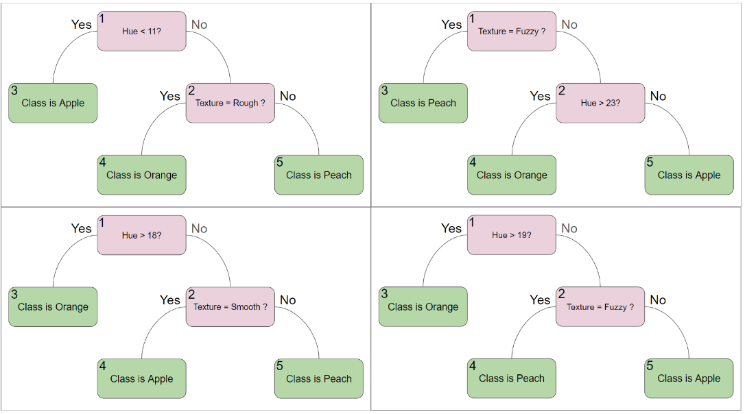
-
Predictions of the 3 data points using the Decision Tree
-
Predictions of the 3 data points using the Random Forest
Question 2 (2 points)
Creating a Random Forest in scikit-learn is very similar to creating a Decision Tree. The main difference is that you will be using the RandomForestClassifier class instead of the DecisionTreeClassifier class.
Please load the Iris dataset, scale it, and split it into training and testing sets using the below code.
import pandas as pd
from sklearn.preprocessing import StandardScaler
from sklearn.model_selection import train_test_split

df = pd.read_csv('/anvil/projects/tdm/data/iris/Iris.csv')
X = df.drop(['Species','Id'], axis=1)
y = df['Species']

scaler = StandardScaler()
X_scaled = scaler.fit_transform(X)

X_train, X_test, y_train, y_test = train_test_split(X_scaled, y, test_size=0.2, random_state=20)

y_train = y_train.to_numpy()
y_test = y_test.to_numpy()
Creating a random forest in scikit is just as simple as creating a decision tree. You can create a random forest using the below code.
from sklearn.ensemble import RandomForestClassifier

forest = RandomForestClassifier(n_estimators=100, random_state=20)
forest.fit(X_train, y_train)
Random forests have 1 additional parameter compared to decision trees, n_estimators. This parameter simply controls the number of trees in the forest. The more trees you have, typically the more robust your model will be. However, having more trees leads to longer training and prediction times, so you will need to find a balance.
Let’s see how it performs with 100 n_estimators by running the below code.
from sklearn.metrics import accuracy_score
y_pred = forest.predict(X_test)
accuracy = accuracy_score(y_test, y_pred)

print(f'Model is {accuracy*100:.2f}% accurate')
If you remember from the previous project, one of the benefits of Decision Trees is their interpretability, and the ability to display them to understand how they are working. In a large random forest, this is not quite as easy considering how many trees are in the forest. However, you can still display individual trees in the forest by accessing them in the forest.estimators_ list. Please run the below code to display the first tree in the forest.
from sklearn.tree import plot_tree
import matplotlib.pyplot as plt

plt.figure(figsize=(10,7))
plot_tree(forest.estimators_[0], filled=True)
Since we are able to access individual trees in the forest, we can also simply use a single tree in the forest to make predictions. This can be useful if you want to understand how a single tree is making predictions, or if you want to see how a single tree is performing.
-
Accuracy of the Random Forest model with 100 n_estimators
-
Display the first tree in the forest
Question 3 (2 points)
Similar to investigating the Decision Tree’s parameters in project 7, let’s investigate how the number of trees in the forest affects the accuracy of the model. Additionally, we will also measure the time it takes to train and test the model.
Please create random forests with 10 through 1000 trees, in increments of 10, and record the accuracy of each model and time it takes to train/test into lists called accuracies and times, respectively. Plot the number of trees against the accuracy of the model. Be sure to use a random_state of 13 for reproducibility.
Code to display the accuracy of the model is below.
import matplotlib.pyplot as plt

plt.plot(range(10, 1001, 10), accuracies)
plt.xlabel('N_Estimators')
plt.ylabel('Accuracy')
plt.title('Accuracy vs N_Estimators')
Code to display the time it takes to train and test the model is below.
import matplotlib.pyplot as plt

plt.plot(range(10, 1001, 10), times)
plt.xlabel('N_Estimators')
plt.ylabel('Time')
plt.title('Time vs N_Estimators')-
Code to generate the data for the plots
-
Graph showing the number of trees in the forest against the accuracy of the model
-
Graph showing the numebr of trees in the forest against the time it takes to train and test the model
-
What is happening in the first graph? Why do you think this is happening?
-
What is the relationship between the number of trees and the time it takes to train and test the model (linear, exponential, etc)?
Question 4 (2 points)
Now, let’s look at our Extra Trees model. Creating an Extra Trees model is the same as creating a Random Forest model, but using the ExtraTreesClassifier class instead of the RandomForestClassifier class.
from sklearn.ensemble import ExtraTreesClassifier

extra_trees = ExtraTreesClassifier(n_estimators=100, random_state=20)
extra_trees.fit(X_train, y_train)
Let’s see how it performs with 100 n_estimators by running the below code.
from sklearn.metrics import accuracy_score

y_pred = extra_trees.predict(X_test)
accuracy = accuracy_score(y_test, y_pred)

print(f'Model is {accuracy*100:.2f}% accurate')-
Accuracy of the Extra Trees model with 100 n_estimators
Question 5 (2 points)
It would be repetitive to investigate how n_estimators affects the accuracy and time of the Extra Trees model, as it would be the same as the Random Forest model.
Instead, let’s look into the differences between the two models. The primary difference between these two models is how they select the data to train each tree. Random Forests use bootstrapping to create multiple datasets, while Extra Trees use a random subset of features and data to train each tree.
We can see how important each feature is to the model by looking at the feature_importances_ attribute of the model. This attribute will show how important each feature is to the model, with higher values being more important. Please run the below code to create new Random Forest and Extra Trees models, and diplay the feature importance for each. Then, write your own code to calculate the average number of features being used in each tree for both models.
import matplotlib.pyplot as plt

forest = RandomForestClassifier(n_estimators=100, random_state=20, bootstrap=True, max_depth=4)
forest.fit(X_train, y_train)

extra_trees = ExtraTreesClassifier(n_estimators=100, random_state=20, bootstrap=True, max_depth=4)
extra_trees.fit(X_train, y_train)

plt.bar(X.columns, forest.feature_importances_)
plt.title('Random Forest Feature Importance')
plt.show()

plt.bar(X.columns, extra_trees.feature_importances_)
plt.title('Extra Trees Feature Importance')
plt.show()-
Code to display the feature importance of the Random Forest and Extra Trees models
-
Code to calculate the average number of features being used in each tree for both models
-
What are the differences between the feature importances of the Random Forest and Extra Trees models? Why do you think this is?
Question 6 (2 points)
There is an additional ensemble method we have not yet discussed, known as Boosting. Both the Random Forest and Extra Trees models utilitze something called bootstrap aggregation, 'Bagging' for short. Bagging works by creating multiple models in parallel and averaging their results, each given a slightly different dataset generated through bootstrapping the original. Boosting, on the other hand, works by creating multiple models in sequence. After each model is created, the deficiencies of it will be recorded and used to construct the next model to improve upon those deficiencies. Typically, this can lead to a very very accurate model. However, since it is creating models in sequence with the goal of improving the accuracy based solely on the training data, it is very prone to overfitting.
Scikit-learn provides three boosting models: AdaBoost, Gradient Boosting, and HistGradient Boosting. Each of these models follow the general theory of boosting, but have slightly different ways of improving upon the deficiencies of the previous model.
AdaBoost: AdaBoost works by creating a model, then creating a second model that focuses on the deficiencies of the first model. Specifically, it will focus on high error points in the training data. This allows the model to rapidly improve upon the deficiencies of the previous model, however becomes prone to outliers and noise in the data.
Gradient Boosting: Gradient Boosting works by creating a model, then creating a second model that focuses on the residuals of the first model. These residuals are the difference between the predicted value and the actual value. This allows the model to focus on the errors of the previous model, and can lead to a very accurate model.
HistGradient Boosting: HistGradient Boosting is a newer model that is optimized to work with very large datasets (10,000+ samples). It works by creating a histogram of the data, then works the same as Gradient Boosting.
Because the Iris dataset is relatively small, we will not be using HistGradient Boosting. However, we will be using and comparing AdaBoost and Gradient Boosting.
Please create an AdaBoost model and a Gradient Boosting model using the below code.
|
A fun thing about the AdaBoost model is that it can be used with any model, not just Decision Trees. One argument in its constructor is |
from sklearn.ensemble import AdaBoostClassifier, GradientBoostingClassifier
from sklearn.tree import DecisionTreeClassifier

adaboost = AdaBoostClassifier(estimator=DecisionTreeClassifier(max_depth=2), n_estimators=100, random_state=20)
adaboost.fit(X_train, y_train)

gradient_boost = GradientBoostingClassifier(n_estimators=100, random_state=20, max_depth=2)
gradient_boost.fit(X_train, y_train)

y_pred = adaboost.predict(X_test)
accuracy = accuracy_score(y_test, y_pred)

print(f'AdaBoost is {accuracy*100:.2f}% accurate')

y_pred = gradient_boost.predict(X_test)
accuracy = accuracy_score(y_test, y_pred)

print(f'Gradient Boosting is {accuracy*100:.2f}% accurate')-
Accuracy of the AdaBoost model
-
Accuracy of the Gradient Boosting model
Question 7 (2 points)
In question 3, we looked at how the number of trees in the forest affected the accuracy of the model. In this question, we will look at how the number of trees in the AdaBoost and Gradient Boosting models affect the accuracy of the model.
Please write code to find the accuracy of the AdaBoost and Gradient Boosting models with 10 through 500 trees, in increments of 10. Record the accuracy of each model into lists called ada_accuracies and grad_accuracies, respectively. Additionally, record the training/testing time of each model into lists called ada_times and grad_times, respectively. Plot the number of trees against the accuracy of the model for both models. Be sure to use a random_state of 7 and max_depth of 2 for reproducibility.
Code to graph the accuracy of the models is below.
import matplotlib.pyplot as plt

plt.plot(range(10, 501, 10), ada_accuracies)
plt.plot(range(10, 501, 10), grad_accuracies)
plt.legend(['AdaBoost Accuracy', 'GradientBoost Accuracy'])
plt.xlabel('N_Estimators')
plt.ylabel('Accuracy')
plt.title('Accuracy vs N_Estimators')
Code to graph the time it takes to train and test the models is below.
import matplotlib.pyplot as plt

plt.plot(range(10, 501, 10), ada_times)
plt.plot(range(10, 501, 10), grad_times)

plt.legend(['AdaBoost Accuracy', 'GradientBoost Accuracy'])
plt.xlabel('N_Estimators')
plt.ylabel('Time')
plt.title('Time vs N_Estimators')-
How do the accuracies of the models compare to eachother?
-
How do their training/testing times compare to eachother? Is there something unexpected in the Time with AdaBoost? Why do you think this is happening? (hint: read the scikitlearn documentation, specifically the
n_estimatorsparameter)
Submitting your Work
-
firstname_lastname_project8.ipynb
|
You must double check your You will not receive full credit if your |