401 Project 07 - Classifiers - Decision Trees
Project Objectives
In this project, we will learn about Decision Trees and how they classify data. We will use the Iris dataset to classify the species of Iris flowers using Decision Trees.
Questions
Question 1 (2 points)
Decision Trees are a supervised learning algorithm that can be used for regression and/or classification problems. They work by splitting the data into subsets depending on the depth of the tree and the features of the data. Its goal in doing this is to create simple decision making rules to help classify the data. Because of this, Decision Trees are very easy to interpret, and often used in problems where interpretability is important.
These trees can be easily visualized in a format similar to a flowchart. For example, if we want to classify some data point as a dog, horse, or pig, a Decision Tree may look like this:
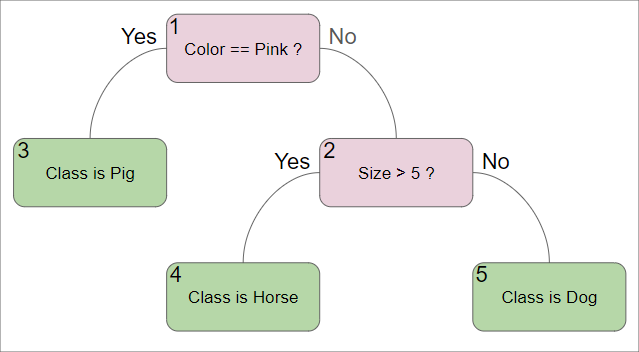
In the above example, then we start at the root node. We then follow each condition until we reach a leaf node, which gives us our classification.
|
In the above example, there is only one condition per node. However, in practice, there can be an unlimited number of conditions per node. These are parameters that can be adjusted when creating the Decision Tree. More conditions in one node can make the tree more complex and potentially more accurate, but it may lead to overfitting and will be harder to interpret. |
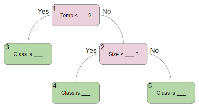
Suppose we have some dataset:
Temp |
Size |
Target |
300 |
1 |
A |
350 |
1.1 |
A |
427 |
90 |
A |
1200 |
1.3 |
B |
530 |
1.2 |
B |
500 |
20 |
C |
730 |
2.1 |
B |
640 |
14 |
C |
830 |
15.4 |
C |
Please fill in the blanks for the Decision Tree below:
-
Answers for the blanks in the Decision Tree. (Please provide the number corresponding to each blank, shown in the top left corner of each box.)
Question 2 (2 points)
For this question we will use the Iris dataset. As we normally do for the classification section, please load the dataset, scale it, and split it into training and testing sets using the below code.
import pandas as pd
from sklearn.preprocessing import StandardScaler
from sklearn.model_selection import train_test_split

df = pd.read_csv('/anvil/projects/tdm/data/iris/Iris.csv')
X = df.drop(['Species','Id'], axis=1)
y = df['Species']

scaler = StandardScaler()
X_scaled = scaler.fit_transform(X)

X_train, X_test, y_train, y_test = train_test_split(X_scaled, y, test_size=0.2, random_state=20)

y_train = y_train.to_numpy()
y_test = y_test.to_numpy()
We can create a Decision Tree classifier using scikit-learn’s DecisionTreeClassifier class. When constructing the class, there are several parameters that we can set to control their behavior. Some examples include:
-
criterion: The function to measure the quality of a split. Supported criteria are "gini" for the Gini impurity and "entropy" for the information gain. -
max_depth: The maximum depth of the tree. If None, then nodes are expanded until all leaves are pure or until all leaves contain less thanmin_samples_splitsamples. -
min_samples_split: The minimum number of samples required to split an internal node. -
min_samples_leaf: The minimum number of samples required to be at a leaf node.
In this project, we will explore how these parameters affect our Decision Tree classifier. To start, let’s create a Decision Tree classifier with the default parameters and see how it performs on the Iris dataset.
from sklearn.tree import DecisionTreeClassifier
from sklearn.metrics import accuracy_score

parameters = {
    "max_depth": None,
    "min_samples_split": 2,
    "min_samples_leaf": 1
}

decision_tree = DecisionTreeClassifier(random_state=20, **parameters)
decision_tree.fit(X_train, y_train)

y_pred = decision_tree.predict(X_test)
accuracy = accuracy_score(y_test, y_pred)

print(f'Model is {accuracy*100:.2f}% accurate with parameters {parameters}')-
Output of running the above code to get the model’s accuracy
Question 3 (2 points)
Now that we have created our Decision tree, let’s look at how we can visualize it. Scikit-learn provides a function called plot_tree that can be used to visualize the Decision Tree. This relies on the matplotlib library to plot the tree. The following code can be used to plot a given Decision Tree:
|
The |
from sklearn.tree import plot_tree
import matplotlib.pyplot as plt

plt.figure(figsize=(20,10))
plot_tree(decision_tree, feature_names=X.columns, class_names=decision_tree.classes_, filled=True, rounded=True)
After running this code, a graph should be generated showing how the decision tree makes decisions. Leaf nodes (nodes with no children, ie. the final decision) should have 4 values in them, whereas internal nodes (nodes with children, often called decision nodes) contain 4 values and a condition. These 4 values are as follows:
-
criterion score (in this case, gini): The score of the criterion used to split the node. This is a measure of how well the node separates the data. For gini, a score of 0 means the node contains only one class, and higher scores mean that the potential classes are more mixed.
-
samples: The number of samples that fall into that node after following the decision path.
-
value: An array representing the number of samples of each class that fall into that node.
-
class: The class that the node would predict if it were a leaf node.
Additionally, you can see that every box has been colored. This is done to help represent the class that the node would predict if it were a leaf node, determined by the 'value' array. As you can see, leaf nodes are a single pure color, while decision nodes may be a mix of colors (see the first decision node and the furthest down decision node).
-
Output of running the above code
-
Based on how the tree is structured, what can we say about how similar each class is to each other? Is there a class that differs significantly from the others?
Question 4 (2 points)
The first parameter we will investigate is the 'max_depth' parameter. This parameter controls how nodes are expanded throughout the tree. A larger max_depth will let the tree make more complex decisions but may lead to overfitting.
Write a for loop that will iterate through a range of max_depth values from 1 to 10 (inclusive) and store the accuracy of the model for a given max_depth in a list called 'accuracies'. Then, run the code below to plot the accuracies.
import matplotlib.pyplot as plt

plt.plot(range(1, 11), accuracies)
plt.xlabel('Max Depth')
plt.ylabel('Accuracy')
plt.title('Accuracy vs Max Depth')
As we increase the max_depth, what happens to the accuracy of the model? What is the smallest max_depth that gives the maximum accuracy?
For now, let’s assume that this smallest max_depth for maximum accuracy is the best parameter to use for our model. Please display the decision trees for a max_depth of 1, this optimal max_depth, and a max_depth of 10.
-
Code that creates the 'accuracies' list
-
Output of running the above code
-
As we increase the max_depth, what happens to the accuracy of the model? What is the smallest max_depth that gives the maximum accuracy?
-
Decision Trees for max_depth of 1, the optimal max_depth, and a max_depth of 10
-
What can we say about the complexity of the tree as max_depth increases? Does a high max_depth lead to uninterpretable trees, or are they still easy to follow?
Question 5 (2 points)
In addition to the importance of the 'max_depth' parameter, the 'min_samples_split' and 'min_samples_leaf' parameters also have a profound effect on the Decision Tree. These parameters control, respectively, the minimum number of samples at a node to be allowed to split, and the minimum number of samples that a leaf node must have. When these values are left at their default values (2 and 1, respectively), the Decision Tree is allowed to continue splitting nodes until there is only a single sample in each leaf node. This easily leads to overfitting, as the model has created a path for the exact training data, rather than a general rule for the dataset.
In this question, we will do something similar to what we did in the previous question, however we will do it for both the 'min_samples_split' and 'min_samples_leaf' parameters. For each parameter, we will iterate through a range of values from 2 to the size of our training data (inclusive) and store the accuracy of the model for a given value in a list called 'split_accuracies' and 'leaf_accuracies' respectively. Leave the value for the other parameter at its default. Then, run the code below to plot the accuracies.
plt.plot(range(2, len(X_train)), split_accuracies)
plt.plot(range(2, len(X_train)), leaf_accuracies)
plt.xlabel('Parameter Value')
plt.ylabel('Accuracy')
plt.legend(['Min Samples Split', 'Min Samples Leaf'])
plt.title('Accuracy vs Split and Leaf Parameter Values')-
Code that creates the 'split_accuracies' and 'leaf_accuracies' lists
-
Output of running the above code
-
What can we say about the effect of the 'min_samples_split' and 'min_samples_leaf' parameters on the accuracy of the model? What values of these parameters would you recommend using for this model?
Question 6 (2 points)
To get a bit more technical, we will be looking at the 'criterion' parameter. Previously, we described this as a function used to measure the quality of a split. However, there is a bit more to it than that. scikit-learn supports two criteria for Decision Trees: 'gini' and 'entropy'.
Gini is a function that measures the impurity of a node. Essentially, the decision tree will attempt to minimize the gini impurity of nodes it creates. The mathematical definition of the gini impurity is as follows:
$ \text{Gini} = 1 - \sum_{i=1}^{n} p_i^2 $
Where $p_i$ is the probability of class $i$ in the node. This value can range from 0 to 0.5, where 0 is a node with only one class, and 0.5 is a node with an equal number of each class.
Entropy is a function that measures the information gain of a node. Information gain is a measure of how much we learn about the data through that split. Its formula is defined as follows:
$ \text{Entropy} = \sum_{i=1}^{n} - p_i \log_2(p_i) $
Where $p_i$ is the probability of class $i$ in the node. This value can range from 0 to 1, where 0 is a node with only one class, and 1 is a node with an equal number of each class.
In almost all cases, the two criteria will give very similar results. To understand this better, we will graph the two functions for a range of p values from 1% to 99%. We will assume a binary classification system, so there are only two classes (P(class 1) + P(class 2) = 1).
Write code to generate lists of gini and entropy values for a range of p_i values from 1% to 99%, in 1% increments. Then, plot the two functions on the same graph using the code below.
|
Remember, the valid range of gini values is from 0 to 0.5, while the range of entropy values is from 0 to 1. For this reason, to validly compare their graphs, you will need to double the gini values so they are on the same scale as the entropy values. |
p_values = np.linspace(0.01, 0.99, 99)
plt.plot(p_values, gini_values)
plt.plot(p_values, entropy_values)
plt.xlabel('P(class 1)')
plt.ylabel('Impurity')
plt.legend(['Gini', 'Entropy'])
plt.title('Gini vs Entropy')-
Code that creates the 'gini_values' and 'entropy_values' lists
-
Output of running the above code
-
What can we say about the differences between the Gini and Entropy functions? Computationally speaking, why do most people use Gini over Entropy?
-
In what cases would you recommend using Entropy over Gini?
Submitting your Work
-
firstname_lastname_project7.ipynb
|
You must double check your You will not receive full credit if your |