TDM 19000: Image Processing

Project Objectives

Motivation: Computers cannot interpret images the way humans do. Instead, images must be converted into numerical representations of themselves that capture import visual features. Learning how image embeddings are created and compared allows us to analyze them, and discover patterns in large collections of images.

Context: In this project, students will use the CLIP model to process images and generate image embeddings, compare images using cosine similarity, and use clustering to group visually similar images based on their extracted features

Scope: Image Processing, CLIP, image embedding, clustering

Learning Objectives

Understand how computers represent visual information using numerical feature vectors.
Generate image embeddings using a pre-trained CLIP model.
Compare images based on their similarity scores
Group images based on visually similar characteristics to create clusters

Dataset

/anvil/projects/tdm/data/images/Snails/*

Snails

The Snails folder contains 30 different images of snails - sourced from this Kaggle Agricultural Pests Image Dataset. The original dataset had 500 images of snails, as well as folders focusing on other animals. This subset was selected because it is a nice starting amount of images to work with without getting overwhelming results at the beginning.

The purpose of this dataset is to give us a sampling of images to break down into vectors, so that we can begin learning about embedding images - putting them into a form the computer will understand. Any dataset of images is fine to use; this was one we found interesting because the snails themselves vary in shape, color, species, and size, as well as the backgrounds of the images can be leaves, dirt, conrete, and other surface, while all still focusing on a singular snail to create consistency across the 30 images.

Questions

Question 1 (2 points)

Humans are naturally good at finding patterns and understanding context that causes something to look how it does - humans instantly process visual information. It’s how we make sense of the world.

Computers excel at taking text, and searching, sorting, and analyzing it at high speeds. Much faster than humans can do. But a computer cannot technically "see" an image - it sees a collection of pixels (or RGB values) that make up any image it encounters.

Image processing allows computers to analyze and interpret visual data. This process is done by taking raw visual data, and transforming it into representations of the image that can be analyzed by a computer. These techniques are now commonly combined with machine learning models, in order to identify patterns across large quantities of images at once.

In this project, we will apply image processing and feature extraction techniques to convert a set of images into numeric embeddings, and then create groups based on similarity.

To get started, we will need to download CLIP - a model that comes from OpenAI. This model learns to connect images and text; it can take an image, and tell you what string of text it is similar to. Similar to some other models we’ve worked with, the CLIP model has some pretty sizable files (far too big for our home directory), so we will have to redirect them to the much larger SCRATCH directory:

# In the Terminal !

# Ensure the .cache folder exists
mkdir -p ~/.cache

# Create the target directory
# (Hugging Face is the platform that hosts OpenAI's CLIP models)
mkdir -p $SCRATCH/huggingface

# Create a symbolic link
ln -s $SCRATCH/huggingface ~/.cache/huggingface

In your notebook, run:

%%bash
ls -l ~/.cache/huggingface

…to verify that the huggingface cache is being redirected to SCRATCH. The output should include something similar to this image:

From here, we need to get the CLIP model and processor:

CLIPModel - allows us to encode images
CLIPProcessor - handles resizing, normalization, and format conversion for images.

from transformers import CLIPModel
from transformers import CLIPProcessor

# loads a pretrained CLIP model from Hugging Face
model = CLIPModel.from_pretrained("openai/clip-vit-base-patch32")

processor = CLIPProcessor.from_pretrained("openai/clip-vit-base-patch32")

When importing CLIPProcessor, you may get a long warning message. This is ok to ignore!

Deliverables

1.1 Explain (1-2 sentences) how computers "understand" visual content
1.2 Direct the CLIP model to store downloads in the SCRATCH directory
1.3 Load the model and processor to prepare for image processing

Question 2 (2 points)

Now we can actually begin working with the model, and have it process some images.

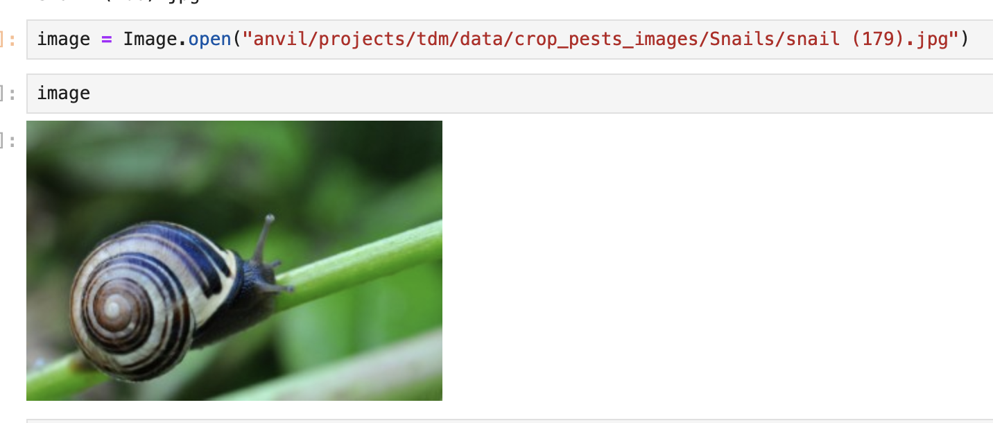
From the 'Snails' folder, choose one image to read in (using Image.open) and view, as done below.

import os

folder_path = "/anvil/projects/tdm/data/images/Snails"

# print the names of the images
for filename in os.listdir(folder_path):
    print(filename)

from PIL import Image

# change the selected image name as needed
my_image = Image.open("/anvil/projects/tdm/data/images/Snails/[your_snail_image].jpg")

my_image

Think of how you might describe the image you’ve just displayed. Some common themes amongst the images in this dataset are:

Very green and leafy background
Snail is fully inside / extended out of its shell
Clear view of shell spiral
Snail on concrete / road

Just as we can think of images by a set of key features, so will the computer…just a bit differently.

For the model to understand what is happening in this image, we must first use the CLIPProcessor (stored as processor in Question 1) to prepare the image. This processor will automatically resize the image, normalize the pixel values to be in a range the model expects, and then convert the image into numerical tensors.

inputs = processor(images=my_image, return_tensors="pt")

inputs

The resulting inputs is a dictionary of tensors, of the shape:

{
    'pixel_values': tensor([...])
}

This is the formatting that the CLIP model expects and knows how to handle as input.

From this point, we then need the model to take the processed image, and convert it into a numercial feature vector - an embedding - that represents the image. This is the model’s way of storing the meaning of what is in the image.

# break the dictionary up into keyword arguments
image_features = model.get_image_features(**inputs)

image_features stores the important parts of the image that make it itself and not any other image.

The result is an embedding that does not make too much sense to us when viewed. But it is actually quite useful for the model. This vector will allow us to make similarity comparisons between multiple images in the future.

# normalize the features to ensure the magnitude doesn't matter
normalized_img_feats = image_features / image_features.norm(dim=-1, keepdim=True)

Deliverables

2.1 Read in an image from the Snails dataset folder, and display it. What are some key features you notice about the image?
2.2 Convert the image into a dictionary of tensors
2.3 Unpack the dictionary (inputs) to find keyword arguments
2.4 Explain (2-3 sentences) how we are using processor and model to make the image model-friendly

Question 3 (2 points)

If we wanted to compare a group of images and decide which were the most similar, sometimes it is easy to do. In this group, it would be the two images of snails:

snail (179) bike 207 snail (103) cat.1

But in a group with very visually similar images, it is a bit harder for us to just look and know:

snail (261) snail (304) snail (262)

All three snails look very similar.

The CLIP model is able to compare how similar images are based on the values in their feature vectors. We will build a loop to read in every image of the Snails folder. For each image, it will be important to make sure that it goes through processor and model so the key description features get stored correctly.

Here is the base template to fill out (with help from the lines we built in Question 2 when processing just 1 image):

# lists to contain the names of the files and the image vectors
filenames = []
features = []

folder = "" # Insert the filepath to the 'Snails' folder

for file in os.listdir(folder):
    if file.endswith(".jpg"):
        path = os.path.join(folder, file)

        with Image.open(path) as image:
            # Define 'inputs' to be the result of running processor on 'image'
            # (so processor will be run on each image)
            # Return the images in a format that CLIP can process
            inputs = ......


        with torch.no_grad():
            # 'image_features' should take the processed images and use
            # model to convert them into embeddings
            # to store what each images "means"
            image_features = ......

        # normalize the image features
        normalized_img_feats = ......

        features.append(feats)
        filenames.append(file)

        print(file)

Print the length of features to ensure that it contains all 30 snail images.

Use combined_features = torch.cat(features, dim=0) to take the list of individual image vectors - each image has its own vector - and combine them into one big tensor. Each row of combined_features represents one image embedding.

For this project, we will use cosine similarity to compare how similar the images are. To start very simply, compare the just two images to find their similarity.

# compare image #0 to image #1
first_similarity = torch.matmul(features[0], features[1])

print(first_similarity)

In cosine similarity, there are three score categories:

-1 - items are dissimilar
0 - items are neutral
1 - items are identical

The similarity scores between the images will follow these patterns.

Deliverables

3.1 How might the CLIP model decide that the three images of snails (shown above) are more similar to each other than to an image of a bike or a cat?
3.2 Read in the 30 snail images and extract a feature vector for each
3.3 Combine the vectors into one total list of vectors
3.4 Show the similarity score of image #0 to image #1. Are these two images dissimilar, neutral, or similar?

Question 4 (2 points)

To find the similarity of each image to every single other image, you can do 'similarities = torch.matmul(features, features.T)'. Printing out similarities would display a tensor containing a vector for each image. Each vector would contain 30 values - 30 images, scoring the similarity to each of the other 29 images and themself. This is very hard to interpret.

To help with this, we can make a heatmap to visually show these similarity scores:

import matplotlib.pyplot as plt
import seaborn as sns

sns.heatmap(similarities.numpy(), xticklabels=filenames, yticklabels=filenames)
plt.show()

On the heatmap, there is a near-white diagonal line that shows the images that are 100% similar to each other - this only occurs on each image vs. itself.

If we wanted to actually look at the images that are scored as the most similar, we would first have to ignore the scores along this diagonal line, as it doesn’t tell us much of anything. There are a few different ways this could be done. We will simply set the diagonal (full of cosine similarity '1' values) so that each value is '0.7'.

In cosine similarity, -1 is used to represent items that are specifically opposite from each other. We could have set the diagonal values here to be -1, so that these scores would never show up as the most similar cases in our analysis. However, the lowest similarity score here is 0.7355 (found using 'similarities.min()'), and setting values of -1 would shift the color gradient too dramatically for any other values to have much meaning (img 2. below). So you should use 'similarities.fill_diagonal_(0.7)', to set the self-comparisons along the diagonal to be scored as 0.7.

Original Scores of 1 Scores of 0.7

(Left to right: Original heatmap of similarity scores; Similarity scores with exact matches set to -1; Similarity scores with exact matches set to 0.7)

With the self-scoring image pairs out of the way, we can now find the pairs of images with the highest similarity scores.

# turn similarities (dictionary of vectors) into a 1D list
# then find the 10 largest similarity values
values, indices = torch.topk(similarities.flatten(), k=10)


# converts the flat indices back into (row, column)
# ( this is reversing the calculations from .flatten() )
pairs = [(idx.item() // len(filenames), idx.item() % len(filenames)) for idx in indices]

# for each item pairing of i and j, print the similarity score
for i, j in pairs:
    print(f"{filenames[i]} & {filenames[j]} are of similarity = {similarities[i, j]}")

filepath = "/anvil/projects/tdm/data/images/Snails"

for i, j in pairs:
    if i < j:
        print(f"\n{filenames[i]} & {filenames[j]} are of similarity = {similarities[i, j]}")

        img1 = Image.open(f"{filepath}/{filenames[i]}")
        img2 = Image.open(f"{filepath}/{filenames[j]}")

        fig, axes = plt.subplots(1, 2, figsize=(6, 3))

        axes[0].imshow(img1)
        axes[0].set_title(f"{filenames[i]}")
        axes[0].axis("off")

        axes[1].imshow(img2)
        axes[1].set_title(f"{filenames[j]}")
        axes[1].axis("off")

        plt.show()

When displaying the images, we use 'if i < j:' inside of the initial for loop. If you look at where we printed the similarity scores of the top image pairs, each set of two lines are the same images, just with image i and image j switched:

snail (339).jpg & snail (179).jpg are of similarity = 0.9496893286705017
snail (179).jpg & snail (339).jpg are of similarity = 0.9496893286705017

Deliverables

4.1 What images (from the initial cosine similarity scores heatmap) are similar? Which are dissimilar?
4.2 Replace the values where the cosine similarity score was 1, and make them each 0.7. How does this change the heatmap?
4.3 Show the image pairings with the top 5 similarity scores.

Question 5 (2 points)

We have found which pairs of images are the most similar. This is useful for direct comparison. But what if we want to find a lot of images that are similar? Or if we would like to divide up an entire folder of images based on similarity?

Clustering is an unsupervised machine learning technique that groups pixels in images based on similar characteristics - this can be color, intensity, or other features in an image. The result of this is clusters (groups) of images that are all similar to each other in some overarching way.

To break up the folder 'Snails' that contains 30 images, we will:

Create 3 clusters for image groups
Label each image based on the features found in its embedding
Apply the label directly to each file name

from sklearn.cluster import KMeans

labels = []

kmeans = KMeans(n_clusters=3, random_state=42).fit(features.numpy())
for idx, label in enumerate(kmeans.labels_):
    print(f"{filenames[idx]} -> Cluster {label}")
    labels.append([filenames[idx], label])

To sort the images based on their cluster, we will create three cluster groups:

from collections import defaultdict

# Initialize a dictionary where key=cluster, value=list of filenames
cluster_groups = defaultdict(list)

for fname, cluster in labels:
    cluster_groups[cluster].append(fname)

To view what files are in each cluster group, use 'print(cluster_groups[__])'.

i.e. to view the files in cluster 0, print(cluster_groups[0]), …, switching the number accordingly.

Looking at the names of the files is good, but it would be cool to actually see the sort of images that got sorted into each cluster.

# !!!!!!!!
# change this [0] according to if you want to show cluster 0, 1, or 2.
my_cluster = cluster_groups[0]

# number of images per row
cols = 4
# calculate number of rows
rows = (len(my_cluster) + cols - 1) // cols

plt.figure(figsize=(cols*3, rows*3))

for i, fname in enumerate(my_cluster):
    path = os.path.join(folder, fname)
    img = Image.open(path)

    plt.subplot(rows, cols, i+1)
    plt.imshow(img)
    plt.axis('off')
    plt.title(fname, fontsize=8)

plt.tight_layout()
plt.show()

Make sure to run the above code for each of the clusters 0, 1, and 2.

Deliverables

5.1 Create clusters to sort the images into
5.2 Show the names of the images within each cluster group (there are three groups)
5.3 Show the images within each cluster groups (three sets of images)
5.4 What main characteristics are you noticing of the images in each cluster?

Submitting your Work

Once you have completed the questions, save your Jupyter notebook. You can then download the notebook and submit it to Gradescope.

Items to submit

firstname_lastname_project[].ipynb

You must double check your .ipynb after submitting it in gradescope. A very common mistake is to assume that your .ipynb file has been rendered properly and contains your code, markdown, and code output even though it may not. Please take the time to double check your work. See here for instructions on how to double check this.

You will not receive full credit if your .ipynb file does not contain all of the information you expect it to, or if it does not render properly in Gradescope. Please ask a TA if you need help with this.