Interactive Plots
Plotly Express (px)
Plotly Express is module inside of the plotly library. It allows the user to make interactive plots, which includes but is not limited to maps, and animations. You can play with color; themes and it even comes with preloaded data sets if you want to test and play around with data.
Bubble Chart Map
We must first load in the data and clean it using Pandas We are going to use public data from Australia that maps out the public toilets across the country and a checklist of the amenities at each location.
import pandas as pd
#importing our csv into pandas
ToiletsAU = pd.read_csv("depot/datamine/etc/toiletmapexport_220501_074429.csv")
#looking at the first 5 rows of our data frame
ToiletsAU.head()
The function 'head' looks at the first 5 rows of your data, it also allows you to see how many columns are in your dataset. This is important because we want to see what information is in the data frame and be able to clean it up.
There are two columns that hold NAN values. We want to get rid of those columns as they are not beneficial to us.
#drops the columns that have NaN values from our dataset
ToiletsAU.drop(columns=["AddressNote", "ToiletNote"], inplace = True)
ToiletsAU
Looking at this data, it is a good time to try and play around with what you could potentially be looking at, if we wanted to see the percentage of states that have toilets with parking access and create a bar graph then we can do this:
#finding the mean or % of the states in each column
ToiletsAU.groupby(["State"]).mean()
#creating a  varaible that shows the % of each state with toilets that have parking
to_plot= ToiletsAU.groupby(["State"]).mean()["Parking"]
import plotly.express as px
fig = px.bar(to_plot)
fig.show()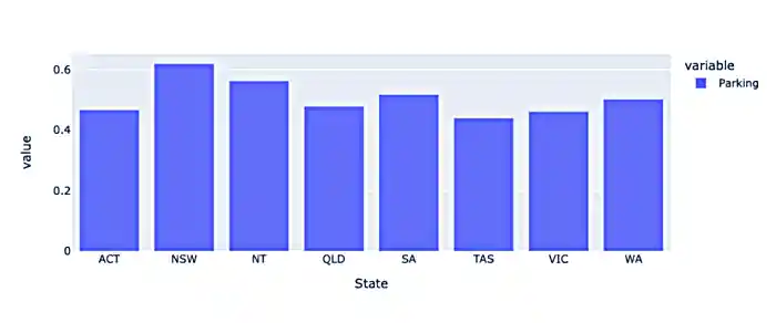
I also spent a lot of time just checking out the data, feel free to do the same, here are some scripts that I ran just to get a better idea of the different numbers and what I was going to plot.
#totaling the number of accessible toilets per town
sum_accessible_toilets_town= ToiletsAU.groupby(["Town"]).sum()["Accessible"]
print(sum_accessible_toilets_town)
#totaling the number of accessible toilets per state
sum_accessible_toilets_state= ToiletsAU.groupby(["State"]).sum()["Accessible"]
print(sum_accessible_toilets_state)#find the maximum value
max_states = sum_accessible_toilets_state.max()
print(max_states)#Find the maximum value
max_town = sum_accessible_toilets_town.max()
print(max_town)#find total number of toilets
total_toilets = len(ToiletsAU.index)
print(total_toilets)#find the total number of accessible toilets
accessible_toilets = ToiletsAU['Accessible'].sum()
print(accessible_toilets)#Grouping by state and counting
ToiletsAU.groupby(["State"]).count()#regrouping the catagories and then finding the sum of each column
regroup = ToiletsAU.groupby(["State", "Town"]).sum().reset_index()
print(regroup)Next, I wanted to take all the data that I had examined and try out creating a bubble scatter plot to show more information
#setting up a scatter plot to see what the information looks like
fig = px.scatter(regroup, x="State", y="Accessible")
fig.show()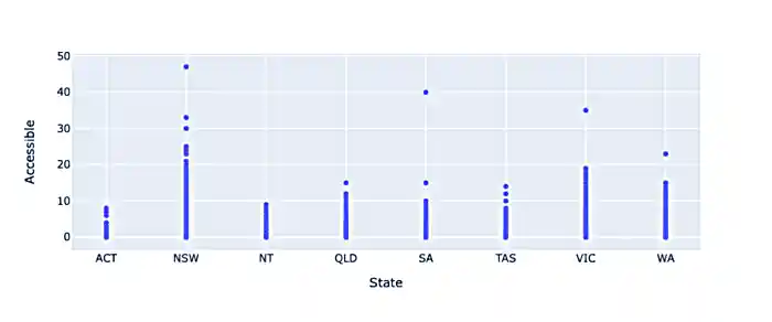
Next, I wanted to take all the data that I had examined and try out creating a bubble scatter plot to show more information
fig = px.scatter(regroup, x="Accessible", y="ParkingAccessible", color="State", size="Shower", size_max=60)
fig.show()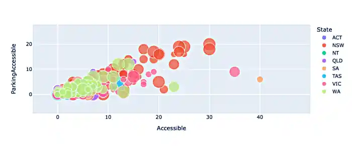
Creating a bubble scatterplot allows for more access to information; but how great would it be to have an immediate understanding of the information just by looking at a map. In order to do this I will need to group by State and Latitude and Longitude
regroup = ToiletsAU.groupby(["State", "Latitude", "Longitude"]).sum().reset_index()
regroup
#sum of states and then reset the index and also specifing which row and which column we want
to_merge = ToiletsAU.groupby("State").sum().reset_index().loc[:,("ParkingAccessible", "State")]
to_merge
#merging indexes
new_regroup = regroup.merge(to_merge, on="State", how="left")
new_regroup
Now we can take our info and create a bubble map
regroup['country'] = "australia"
fig = px.scatter_geo(new_regroup, lat="Latitude", lon="Longitude", size="ParkingAccessible_y", center={'lat':-35.875892 , 'lon': 148.985187} )
fig.update_layout(
        geo = dict(
            projection_scale=5, #this is kind of like zoom
            center=dict(lat=-23.52152, lon=134.3974), # this will center on the point
        ))
fig.show()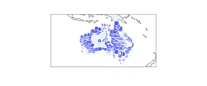
How cool is that? Really this is all about looking at data and finding different ways to create interactive graphs and charts, to help visualize the story that we are telling. In the end this map shows that where the accessible toilets are, and if they have accessible parking. Feel free play around in Plotly Express using different ways to visualize data!
This Exploratoray Data Analysis page also has some really great information on how to look at your data.
|
Plotly Express does allow for color modifications which we did not do in this exercise. If you do not assign color values Plotly Express will automatically assign them. Using the automation, however does not take into consideration what colors may be most effective for those that are blind or low vision. |