Introduction
We are going to continue to see if we can uncover clues that will help the investigators uncover the murderer.
To do this we are going to use some controversial data, phone records.
In this case we simulated the data as an example, but it is important to note that many companies and applications do track location data for their users.
Geospatial Data
Today we get to work with a really interesting type of data, geospatial data.
This data looks very similar to the data that we’ve used so far with one important difference. This data has information about the location in the world.
Location can be found in different ways. In this case we have latitude and longitdue.
The other cool part about geospatial data is that we have many open-source options. For this part of the process we’ll start with the DC street map data that is provided by the city.
Practice Exercises
-
We will start by importing all the different Python packages that we will need and taking a look at the DC street map data.
Click to see solution
import pandas as pd
import geopandas as gpd
import matplotlib.pyplot as plt
import random
import numpy as np

from datetime import datetime, timedelta
from shapely.geometry import Point, Polygon
dc_streets = gpd.read_file('../data/dc_roads/Roads.shp')fig, ax = plt.subplots(figsize = (15,12)) dc_streets.plot(ax = ax) plt.show() plt.close('all')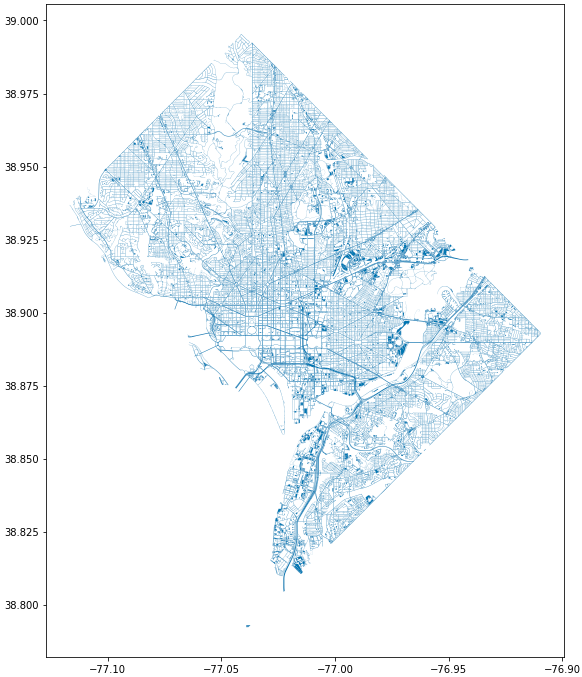 Figure 1. High Level View of the Streets of DC
This is a very interesting map, but it’s hard to read. We will do something about that, but first we can take a look at the raw data as well.
-
Let’s print out the raw data to better understand the dataset.
Click to see solution
print(dc_streets.head())FEATURECOD DESCRIPTIO CAPTUREYEA CAPTUREACT GIS_ID OBJECTID \ 0 1060 Alley 2015-04-24 E RoadPly_1 1 1 1065 Paved Drive 2015-04-24 E RoadPly_2 2 2 1070 Parking Lot 2015-04-24 E RoadPly_3 3 3 1050 Road 2015-04-24 E RoadPly_4 4 4 1050 Road 2015-04-24 E RoadPly_5 5 SHAPEAREA SHAPELEN geometry 0 0 0 POLYGON ((-77.07695 38.92945, -77.07686 38.929... 1 0 0 POLYGON ((-77.07839 38.93672, -77.07839 38.936... 2 0 0 POLYGON ((-77.07602 38.94230, -77.07613 38.942... 3 0 0 POLYGON ((-77.07870 38.94405, -77.07870 38.943... 4 0 0 POLYGON ((-77.07542 38.92373, -77.07543 38.923...
We can see that the DC streets data looks pretty similar to what we’ve been working with.
The biggest difference are the
geometryrows. These are sets of latitude and longitude points that Python understands spatially.This means that we can use these points for different sptial functions, like finding distance.
First though, lets cut down our huge map to our area of interest. We’ll define our general area of interest around the Mall using Google Maps.
-
Let’s cut down our map to a smaller scale.
Click to see solution
area_of_interest = [-77.062859, 38.880868, -76.982087, 38.915758]

smaller_map = gpd.clip(dc_streets, area_of_interest)
fig, ax = plt.subplots(figsize = (15,15)) smaller_map.plot(ax = ax) plt.plot(-76.9926056723681, 38.90839920511692, c='orange', marker="*", markersize=30) plt.show() plt.close('all')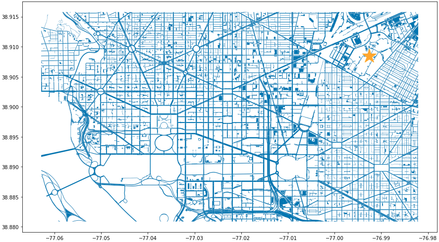 Figure 2. Focused View of DC Streets
 -
Now that we have our smaller map we can take a look at our cell phone data.
Click to see solution
cell_phone_data = gpd.read_file('../data/cell_phone_records.geojson')
print(cell_phone_data.head())
date id lat lon \ 0 2022-05-02 00:17:14.404 0 38.890393 -77.011107 1 2022-05-02 00:27:14.404 0 38.905440 -76.982952 2 2022-05-02 00:37:14.404 0 38.901316 -76.991544 3 2022-05-02 00:47:14.404 0 38.908996 -77.048789 4 2022-05-02 00:57:14.404 0 38.893913 -77.032013 geometry 0 POINT (-77.01111 38.89039) 1 POINT (-76.98295 38.90544) 2 POINT (-76.99154 38.90132) 3 POINT (-77.04879 38.90900) 4 POINT (-77.03201 38.89391)This data looks pretty similar to our DC streets data. It has dates and times as well as the ID for the caller. The most important parts are the
latandloncolumns that we can use to map the caller’s path. -
Let’s map out our data and see what it looks like!
Details
n = len(cell_phone_data['id'].unique()) color = iter(plt.cm.rainbow(np.linspace(0, 1, n))) fig, ax1 = plt.subplots(1, 1, figsize=(15, 8)) smaller_map.plot(ax = ax1) plt.plot(-76.9926056723681, 38.90839920511692, c='orange', marker="*", markersize=30) for i in range(0, cell_phone_data['id'].max()): person = cell_phone_data.loc[cell_phone_data['id'] == i].sort_values(by='date') plt.plot(person['lon'], person['lat'], c=next(color), linestyle='--') plt.show() plt.close('all')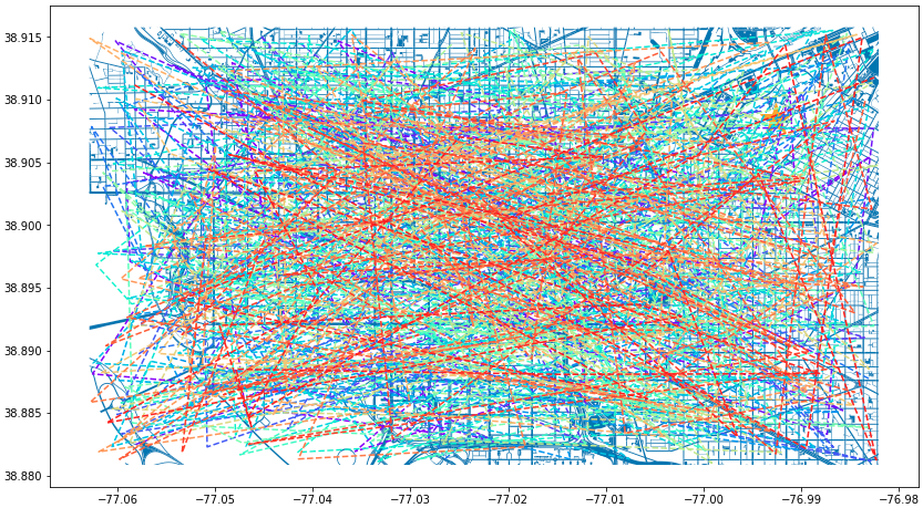 Figure 3. Map of DC with Phone Paths
This is an interesting map, but it’s very noisy. For our next step lets see if we can limit the map to only calls that went near where our victim was found.
In this section you’ll see references to
crswith some odd looking numbers and letters after them likeepsg:4326. These are what are known as coordinate reference systems.Their specific detail is beyond the scope of this workshop, but at a high-level they help convert coordinates to address different ways of looking at the earth.
In our case, we have to convert the CRS' to something that is better for measuring distance in North America.
-
Lets calculate the distance from our victim’s location to all of the lat/lon points that we have in the phone records.
Details
starting_point = gpd.GeoSeries([Point(-77.03718028811417, 38.88978312185629) for i in range(len(cell_phone_data))], crs='epsg:4326')

cell_phone_data = cell_phone_data.to_crs('EPSG:32633')
starting_point = starting_point.to_crs('EPSG:32633')

cell_phone_data['distance'] = cell_phone_data.distance(starting_point)

cell_phone_data['distance_miles'] = cell_phone_data['distance'] * 0.000621371

print(cell_phone_data[cell_phone_data['distance_miles'] < 1])
date id lat lon \ 4 2022-05-02 00:57:14.404 0 38.893913 -77.032013 10 2022-05-02 01:57:14.404 0 38.881946 -77.035672 12 2022-05-02 02:17:14.404 0 38.892572 -77.026673 18 2022-05-02 03:17:14.404 0 38.886712 -77.041343 22 2022-05-02 03:57:14.404 0 38.885509 -77.046967 .. ... .. ... ... 758 2022-05-01 20:30:00.000 25 38.896051 -77.043628 762 2022-05-01 21:10:00.000 25 38.889835 -77.040619 763 2022-05-01 21:20:00.000 25 38.892248 -77.036607 766 2022-05-01 21:50:00.000 25 38.895527 -77.029528 767 2022-05-01 22:00:00.000 25 38.892288 -77.033660 geometry distance distance_miles 4 POINT (-6130636.381 10277516.684) 1016.764717 0.631788 10 POINT (-6132711.509 10278137.551) 1395.192331 0.866932 12 POINT (-6130913.298 10276796.415) 1526.595396 0.948582 18 POINT (-6131829.871 10278869.453) 787.591153 0.489386 22 POINT (-6131997.658 10279654.020) 1542.512663 0.958473 .. ... ... ... 758 POINT (-6130170.922 10279090.606) 1415.560118 0.879588 762 POINT (-6131286.540 10278738.958) 473.128919 0.293989 763 POINT (-6130893.552 10278164.074) 441.023789 0.274039 766 POINT (-6130371.878 10277159.468) 1459.603516 0.906955 767 POINT (-6130909.354 10277758.863) 654.950097 0.406967 -
Now we can use visualizations to see where a good cutoff point may be for "close" to our victim.
Details
fix, ax1 = plt.subplots(1, 1, figsize=(8,6)) ax1 = plt.hist(cell_phone_data['distance_miles'], bins=25) plt.show() plt.close('all')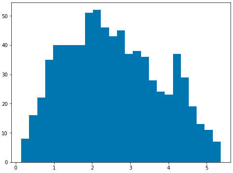 Figure 4. Histogram of Distance from Point of Interest
 -
This helps, but let’s look at distances less than 1 mile.
Details
fix, ax1 = plt.subplots(1, 1, figsize=(8,6)) ax1 = plt.hist(cell_phone_data.loc[cell_phone_data['distance_miles'] < 1]['distance_miles'], bins=25) plt.show() plt.close('all')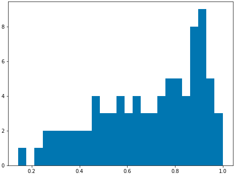 Figure 5. Histogram of Distance from Point of Interest < 1 Mile
Based on the histogram it looks like we could use half a mile as a good cutoff.
-
Using half a mile lets see what our updated map looks like.
Details
id_of_interest = cell_phone_data.loc[cell_phone_data['distance_miles'] < 0.5]['id'].unique()
cell_phone_data['close_point'] = cell_phone_data['id'].isin(id_of_interest)
cell_phone_data_reduced = cell_phone_data.loc[cell_phone_data['close_point'] == True].reset_index()
n = len(cell_phone_data_reduced['id'].unique()) color_1 = iter(plt.cm.rainbow(np.linspace(0, 1, n))) fig, ax1 = plt.subplots(1, 1, figsize=(15, 8)) smaller_map.plot(ax = ax1) plt.plot(-76.9926056723681, 38.90839920511692, c='orange', marker="*", markersize=30) for i in cell_phone_data_reduced['id'].unique(): person = cell_phone_data_reduced.loc[cell_phone_data_reduced['id'] == i].sort_values(by='date') plt.plot(person['lon'], person['lat'], c=next(color_1), linestyle='--') plt.show() plt.close('all')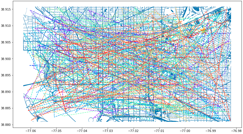 Figure 6. DC Street Map with Distance Filtered Call Routes
We’ve reduced the noise some, but it’s still pretty hard to read.
The investigators told us that due to the location the crime had to take place at nigh. We can use the time of the calls to see if we can reduce our data further.
-
We will extract time and then filter to calls that only happened late at night.
Details
cell_phone_data_reduced['hour'] = cell_phone_data_reduced['date'].apply(lambda x: x.hour)
cell_phone_data_reduced['minute'] = cell_phone_data_reduced['date'].apply(lambda x: x.minute)
cell_phone_data_reduced.head()
index date id lat lon \ 0 0 2022-05-02 00:17:14.404 0 38.890393 -77.011107 1 1 2022-05-02 00:27:14.404 0 38.905440 -76.982952 2 2 2022-05-02 00:37:14.404 0 38.901316 -76.991544 3 3 2022-05-02 00:47:14.404 0 38.908996 -77.048789 4 4 2022-05-02 00:57:14.404 0 38.893913 -77.032013 geometry distance distance_miles \ 0 POINT (-6131415.531 10274679.579) 3588.816997 2.229987 1 POINT (-6128984.462 10270666.938) 7951.698847 4.940955 2 POINT (-6129644.341 10271886.629) 6597.517065 4.099506 3 POINT (-6127856.245 10279670.550) 3739.428950 2.323573 4 POINT (-6130636.381 10277516.684) 1016.764717 0.631788 close_point hour minute 0 True 0 17 1 True 0 27 2 True 0 37 3 True 0 47 4 True 0 57Now that we have
hourandminuteextracted lets filter our data to calls between 11 PM and 4 AM and map them.cell_phone_data_reduced_night = cell_phone_data_reduced.loc[(cell_phone_data_reduced['hour'] > 23) | (cell_phone_data_reduced['hour'] < 4)] id_count = cell_phone_data_reduced_night['id'].unique() print("We have {} late night IDs".format(len(id_count)))We have 7 late night IDs
cell_phone_data['final_id'] = cell_phone_data['id'].isin(id_count)
final_data = cell_phone_data.loc[cell_phone_data['final_id'] == True].reset_index()
n = len(final_data['id'].unique()) color_1 = iter(plt.cm.rainbow(np.linspace(0, 1, n))) fig, ax1 = plt.subplots(1, 1, figsize=(15, 8)) smaller_map.plot(ax = ax1) plt.plot(-76.9926056723681, 38.90839920511692, c='orange', marker="*", markersize=30) for i in final_data['id'].unique(): person = final_data.loc[final_data['id'] == i].sort_values(by='date') plt.plot(person['lon'], person['lat'], c=next(color_1), linestyle='--', label="caller {}".format(i)) plt.legend() plt.show() plt.close('all')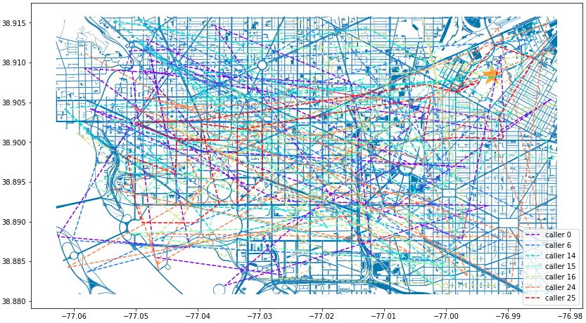 Figure 7. DC Street Map with Calls Filtered by Time
Narrowing our data down to 7 suspects is great!
To help the investigators we can also break each of the 7 calls into its own graph.
-
Let’s create a new vis that has a separate graph for each of the late-night calls.
Details
ids_to_plot = final_data['id'].unique() color_1 = iter(plt.cm.rainbow(np.linspace(0, 1, 7))) fig, axs = plt.subplots(nrows=3, ncols=3, figsize=(25, 20)) for id, ax in zip(ids_to_plot, axs.ravel()): smaller_map.plot(ax = ax, alpha=0.25) single_caller = final_data.loc[final_data['id'] == id] ax.plot(single_caller['lon'], single_caller['lat'], c=next(color_1), linestyle='--') ax.plot(-76.9926056723681, 38.90839920511692, c='orange', marker="*", markersize=30)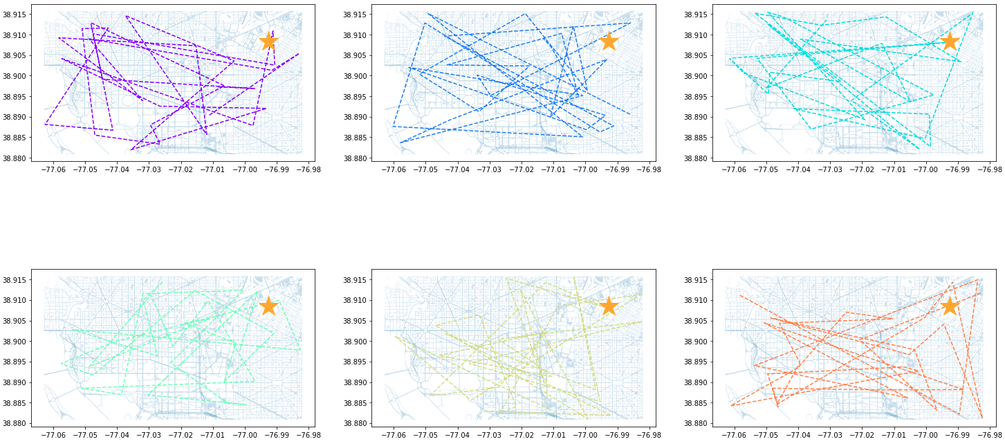 Figure 8. DC Street Map with Individual Calls - Part 1
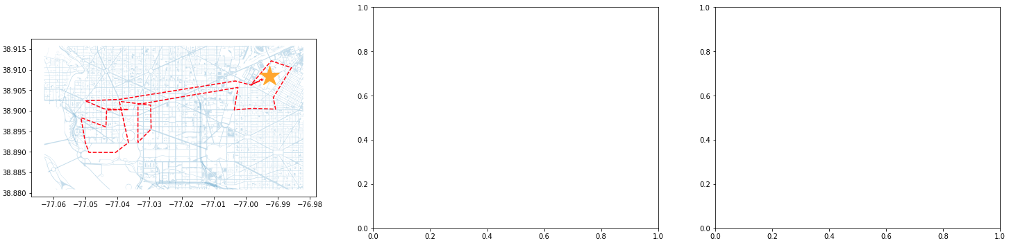 Figure 9. DC Street Map with Individual Calls - Part 2
As a last analysis step we can create an animation that will show the caller’s path through DC.
-
Let’s animate the paths based on
id.Details
from matplotlib.animation import FuncAnimation
from IPython.display import HTML
# We can use this list ot pick the ID that we are interested in. print(final_data['id'].unique())[ 0 6 14 15 16 24 25]
data_subset = final_data.loc[final_data['id'] == 25].reset_index()

fig = plt.figure(figsize=(15, 10))
ax = plt.axes(xlim=(-77.062859, -76.982087), ylim=(38.880868, 38.915758))
line, = ax.plot([], [], lw=2)

x_data = []
y_data = []

def init():
    line.set_data([], [])
    return line,

def animate(i):
    x_data.append(data_subset['lon'][i])
    y_data.append(data_subset['lat'][i])

    line.set_xdata(x_data)
    line.set_ydata(y_data)

    return line

smaller_map.plot(ax = ax, alpha=0.25)
anim = FuncAnimation(fig, animate, frames=len(data_subset), init_func=init, interval=300)

HTML(anim.to_jshtml())
This will create an animation that will display in our browser.
We can update the
final_data.loc[final_data['id'] == 25]ID to animate the different paths.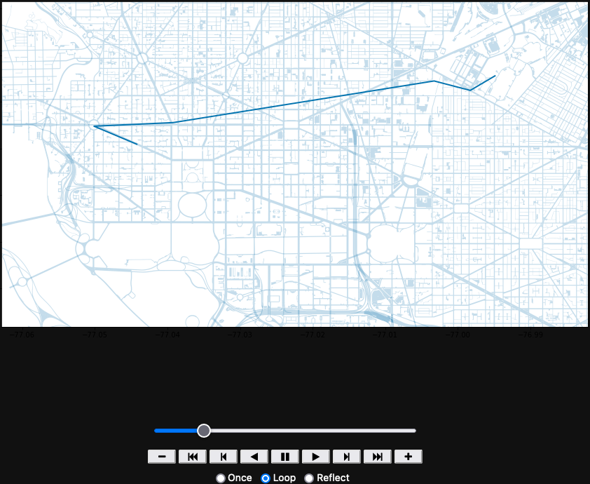 Figure 10. Animation of the Caller’s Path
We can pass these 7 suspects on to our next phase of investigation!